Reviewers Professor
Angappa Gunasekaran
University
of Massachusetts
Department
of Management
North
Dartmouth, MA 02747-2300
USA
Professor Denis R. Towill
Cardiff
University
Department of Maritime
Studies and International Transport
Logistics Systems Dynamics
Group
65-68 Park Place
PO Box 907
Cardiff CF10 3YP
Wales UK
CONTENTS
FIGURES.....................................................................................................................5
TABLES.......................................................................................................................8
NOTATIONS...............................................................................................................9
ABSTRACT................................................................................................................12
1 Introduction............................................................................................... 13
1.1 Research problem context and
formation........................................................... 13
1.2 Justification for the research.............................................................................. 15
1.3 Research strategy and outline of
the report........................................................ 16
1.4 Definitions........................................................................................................ 18
1.5 Delimitations of scope and key
assumptions....................................................... 21
1.6 The structure of the study.................................................................................. 22
2 Research environment and
literature review.................... 23
2.1 Research environment....................................................................................... 23
2.1.1 Background to the research........................................................................ 23
2.1.2 Agility and flexibility approaches in the literature.......................................... 30
2.1.3 Recent research......................................................................................... 33
2.2 Agility and flexibility dimensions......................................................................... 36
2.2.1 Dimensions in the literature......................................................................... 36
2.2.2 Flexibility measurement and performance.................................................... 43
2.2.3 Empirical research on agile manufacturing................................................... 51
2.3 Production dynamics......................................................................................... 55
2.3.1 Structural dynamics of response................................................................. 56
2.4 Conclusions...................................................................................................... 58
3 Agile manufacturing in the
electronics industry
context............................................................................................................ 60
3.1 Overview: electronics
manufacturing environment............................................... 60
3.2 Product availability – value and
cost of time....................................................... 64
3.3 Proposed framework for agility and
flexibility..................................................... 69
3.3.1 Volume flexibility........................................................................................ 70
3.3.2 Mix response flexibility............................................................................... 71
3.3.3 Life cycle flexibility..................................................................................... 73
3.3.4 Technological flexibility............................................................................... 74
3.3.5 Agility measurement................................................................................... 74
3.4 Conclusions...................................................................................................... 79
4 System dynamics models of agile
production...................... 81
4.1 Justification for the methodology........................................................................ 81
4.2 Structural dynamics: demand
magnification and order variations......................... 84
4.2.1 Capacity constraining the system – a flexibility perspective.......................... 91
4.3 Product variety: mix uncertainty
and lot-sizing.................................................... 95
4.3.1 Lead time performance and queuing theory................................................. 97
4.3.2 Lot-sizing................................................................................................. 101
4.3.3 Product availability and dedicated capacity............................................... 104
4.4 Analysing the product life cycles...................................................................... 108
4.5 Conclusions.................................................................................................... 113
5 Analysis of empirical results........................................................ 116
5.1 Procedure of empirical analysis....................................................................... 116
5.2 Industrial Electronics Case Study
– applying the agility/flexibility
framework...................................................................................................... 117
5.2.1 Volume fluctuations in the supply chain..................................................... 119
5.2.2 Mix uncertainty in the chain...................................................................... 121
5.3 Uncertainty in electronics
manufacturing – what flexibility is needed
for agile production?....................................................................................... 125
5.4 Financial analysis of industrial
and consumer electronics manufacturing............. 128
5.4.1 Clustering of companies........................................................................... 130
5.5 Financial performance in
environments............................................................. 135
5.6 Summary of the empirical analysis................................................................... 139
6 Discussion of implication of
research..................................... 142
6.1 Introduction.................................................................................................... 142
6.2 Agility and manufacturing strategy.................................................................... 144
6.3 Proposed approach and supply
elasticity......................................................... 146
6.4 Implications for policy and practice................................................................. 148
7 Conclusions and further research........................................... 152
7.1 Conclusions on each research
question............................................................ 152
7.1.1 Cost effect of response............................................................................ 152
7.1.2 Is agility different depending on the manufacturing environment?................ 158
7.2 Conclusions on the research
problem.............................................................. 160
7.3 Comparison to previous work......................................................................... 161
7.4 Validity and reliability
evaluation – research limitations..................................... 165
7.5 Further research............................................................................................. 166
Acknowledgements..................................................................................... 169
References......................................................................................................... 170
APPENDICES
Appendix 1. Statistical analysis of Finnish electronic
industry........................................ 186
Appendix 2. Details of
multi-machine queue model...................................................... 187
Appendix 3. Source code
for "Forrester Effect"........................................................... 187
Appendix 4. Source code
for "Surge Effect"................................................................ 190
Appendix 5. Source code
for "Capacity in Dynamic Growth"....................................... 191
Appendix 6. Source code
for "Agile Production"......................................................... 193
Appendix 7. Source code
for "Mix flexibility"............................................................... 195
Appendix 8. Source code
for "Dedicated capacity"...................................................... 197
Appendix 9. Cluster
analysis....................................................................................... 198
Appendix 10. Electronic
Contract Manufacturers......................................................... 203
Appendix 11. Source code
for "Supply and demand"................................................... 204
FIGURES
Figure 1. Stella notation – stock, flow and an auxiliary
variable....................................... 10
Figure 2. Stella notation – advanced elements................................................................ 11
Figure 3. Three nodes of research (adapted from Nilsson 1995).................................... 17
Figure 4. Outline of the research (author)....................................................................... 18
Figure 5. US competitive priorities 1988–1996 (Wu 1994)........................................... 27
Figure 6. Declining product life cycles in Siemens AG (von
Braun 1990)........................ 29
Figure 7. Upton's model of flexibility determinants (Upton 1997).................................... 34
Figure 8. Correa's (1994) linkages of change and flexibility
and Upton's (1994)
...... flexibility framework...................................................................................... 42
Figure 9. Classification of flexibility measures (De Toni &
Tonchia 1998: 1605)............. 43
Figure 10. Flexibility and cost curves according to Mills
(1984)..................................... 48
Figure 11. A case of hypothetical flexibility as an investment
curve (Takala 1994)........... 49
Figure 12. Flexibility over product life cycle and demand
profile
(Hutchinson & Sinha
1989).......................................................................... 50
Figure 13. Demand variation has components of trend, season,
cycles
...... and random (Tersine 1985)......................................................................... 54
Figure 14. The order de-coupling point defines the production
type
(Bertrand et al. 1990b)............................................................................... 56
Figure 15. Positioning the planning environments according to
Bartezzaghi &
...... Verganti (1995: 158)................................................................................... 57
Figure 16. Typical production phases in electronics production
process. (author)............ 62
Figure 17. Survey of contract manufacturers: Major challenges
faced when
...... dealing with component manufacturers (Harbert 1997)................................. 64
Figure 18. The value and cost against the lead time (author)........................................... 65
Figure 19. The value of delivery performance (adapted from Houlihan
1987)................. 66
Figure 20. Frequency and accuracy of production forecasts over
forecast
...... horizon used in companies (Gordon & Livingston
1999)............................... 68
Figure 21. Lead times for manufacturing service companies,
including several
market sectors in
electronics (Gordon & Livingston 1999)............................ 68
Figure 22. Ability for response in contract manufacturers (20%
increase in demand)
...... (Gordon & Livingston 1999)........................................................................ 69
Figure 23. The interrelations between agility, flexibility,
response and
...... productivity (author).................................................................................... 76
Figure 24. Efficiency and flexibility are independent components
in
productivity (author)..................................................................................... 78
Figure 25. Economic structure of manufacturing costs (Tseng and
Jiao 1998: 11)........... 79
Figure 26. Updated engineering approach for performance enhancement
of
systems (Pritsker 1997:
779)........................................................................ 83
Figure 27. Forrester Effect simulation in a three-echelon supply
chain
...... (reconstructed from Forrester 1958)............................................................ 85
Figure 28. Demand amplification in the supply chain occurs from
echelon to echelon,
...... and emerges in particular when demand is changing
(author)......................... 86
Figure 29. Some general causes of demand amplification (Houlihan
1987)...................... 87
Figure 30. The Surge Effect model includes four order cycles and
a stable
...... consumption (author)................................................................................... 89
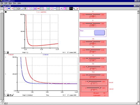
Figure 31. Simulation results of the Surge Effect (author)................................................ 90
Figure 32. Trade-off between delivery performance and cost
efficiency (author)............. 92
Figure 33. Production and supply part from the simulation model
(author)...................... 93
Figure 34. Demand, despatch and inventory (author)..................................................... 93
Figure 35. Financial performance section of the model (author)...................................... 94
Figure 36. Lead time mechanism (author)...................................................................... 94
Figure 37. Productivity with 90–10 and 10–90 cost structures
(author).......................... 96
Figure 38. System time as function of utilisation (arrival rate
/ service rate) (t=1)
...... (author)....................................................................................................... 98
Figure 39. Effects of lot sizing decision on lead time with the
utilisation parameters
...... of 0.4, 0.2 and 0.8 (author)......................................................................... 99
Figure 40. System time as a function of service rate, arrival
rate and number of
...... machines (author)...................................................................................... 101
Figure 41. Lead time as a function of lot size (author)................................................... 103
Figure 42. Unit cost as a function of lot sizes (author)................................................... 103
Figure 43. Standard deviation of inter-arrival rate vs. lead
time (author)........................ 104
Figure 44. Standard deviation of inter-arrival rate vs. unit
cost (author)......................... 104
Figure 45. Analytical structure of volume flexibility (author).......................................... 106
Figure 46. Structure for dividing capacity into availability
groups (author)..................... 107
Figure 47. Lead times for three availability groups (author)........................................... 108
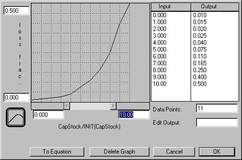
Figure 48. Mechanism of s-shaped learning curve in new product
introduction
...... (author)...................................................................................................... 109
Figure 49. S-shaped learning curve in new product introduction (author)...................... 110
Figure 50. Ramp-up to volume and lead time for order fulfilment
(author)..................... 111
Figure 51. The capacity addition process in a case of expanding
sales and markets
...... (reconstructed from Forrester 1968)........................................................... 112
Figure 52. Capacity restricting the market share development
(author)......................... 113
Figure 53. Summary of model conclusions for volume, mix and life
cylcle
...... uncertainties (author)................................................................................. 115
Figure 54. Order mechanism of the case supply chain (author)..................................... 118
Figure 55. Time analysis of supply chain (author)......................................................... 118
Figure 56. Cumulative volume for board types and histogram of
order sizes
(author)..................................................................................................... 123
Figure
57. Estimate of worldwide contract
manufacturers sales (McHale 1999)............ 129
Figure 58. Inventory parameters tied in the production process
(author)....................... 130
Figure 59. Scatter of proportion of materials and human
resources from sales
...... (author)...................................................................................................... 133
Figure 60. Phases of Electronics Manufacturing Service companies
(author)................. 134
Figure 61. Summary of case based empirical analysis (author)...................................... 140
Figure 62. Summary of
clustering and financial analyses (author)................................. 141
Figure 63. Agility, flexibility and enabling factors (author)............................................. 144
Figure 64. Approaches to trade-off and strategy thinking (Slack
1998)........................ 145
Figure 65. Demand and supply – an economic model
(Richmond and Peterson
1997).................................................................. 147
Figure 66. The economic stabilising effect (author)....................................................... 147
Figure 67. Variations in capacity utilisation increase the cost
of risk (author)................. 154
Figure 68. Generic capacity structure. All idle capacity is not
non-productive
.... (author)..................................................................................................... 158
Figure 69. Production control and agility dimensions are
different in each
...... environment
(author)................................................................................. 160
TABLES
Table 1. Generic manufacturing strategies (Gerwin 1993: 397)....................................... 24
Table 2. The top five competitive priorities in the next five
years (De Meyer 1992),
...... flexibility related priorities are in italics.............................................................. 25
Table 3. Empirical data on lead time reduction (Mason-Jones
and Towill 1999)............. 26
Table 4. Comparison of proposed flexibility measures (author)....................................... 58
Table 5. A comparison of model type (Wu 1994: 219).................................................. 82
Table 6. Summary of flexibility dimensions and their enabler
(author)............................ 115
Table 7. Estimated reduction in factory overhead costs when
responding to ramped
...... output, according to Towill, Naim & Wikner (1992: 10)................................ 119
Table 8. Order magnification in the case supply chain. Demand
variation is calculated
......
as a standard deviation of
demand for a period of one year from an ERP
system (author)............................................................................................. 121
Table 9. Initial status of production system and after
reconsidering the lot-sizes,
calculated with the Mix
Flexibility model (author)........................................... 124
Table 10. Summary of 10 descriptive cases (author).................................................... 127
Table 11. Stereotypes of electronics manufacturing (author)......................................... 127
Table 12. Consumer segment uncertainties and enabling factors
(author)....................... 128
Table 13. Professional segment uncertainties and enabling
factors (author).................... 128
Table 14. Clustering analysis for the sample EMS companies
based on cost
...... structure (author)........................................................................................ 131
Table 15. Inventory and cost structure for EMS categories
(author)............................. 136
Table 16. Top high mix and high volume EMS (author)................................................ 138
Table 17. Operating margin and product mix in some Finnish EMS
firms (author)......... 138
Table 18. Managerial recommendations for EMS agile manufacturing
(author).............. 151
Table 19. Interpretation of agility/flexibility values (author)............................................ 156
Table 20. Summary of comparison to previous work (author)...................................... 163
NOTATIONS
Notation used in formal
analysis
Lq Average number
of jobs waiting (in the buffer) for service
q, ca Inter-arrival time
SCV
N Maximum number of jobs allowed in
the system
l Mean arrival
rate (units/time)
m Mean service
rate (units/time)
t Mean service
time, mean time to process a job (including setup time and process time for all
pieces in the lot)
p Mean time
between arrivals of jobs to the work centre
m Number of
machines in the work centre
s, cs Service time SCV
r Utilisation of
a machine
M Number of
service channels
S System time.
Average time spent by a job in the system from arrival to departure
U Utilisation of
work centre (fraction of time spent working on a job)
W Average time a job spends
waiting (in the buffer) before beginning a service
L Actual load
C Capacity factor
R Required capacity
a Number of workforce in a
system
q Lot size
k Flexibility of a system
spaced structure
D Delivery lead
P Total available lead time
for a product
Bj Available time for machine type j per day
xi Total number produced per day for product type i
tij Machine
time for type j per unit used for
product type i
VF Volume
flexibility
VR Profitability
range
Cmax Maximum
capacity of the system
a Number of
capacity units required per parts produced
NB Lower
limit of profitable production range
EF Expansion
flexibility
EMVF Flexible
option
EMVC Conventional
option
D1, D2,… ,Dm Demand
set
p Contribution
of the product
kC Unit acquisition
cost of conventional capacity
kF Unit acquisition
cost of conventional capacity
CC Conventional capacity
purchased
F Machine M's
flexibility in proportion to its task T,
r Working
condition for a machine
e(r) The normal
condition work performance
E Maximum value
of e(r) within a changing range -r to r
i Average number of operations
Kei The effective capacity of machine i
qj Average quantity over a given period of time
tii Average operation time
a Degree of similarity of parts in material flow
hi Degree of utilisation (load)
n The number of
dissimilar products
duri The duration of the setup for each
product i.
cb Machine flexibility, Nilsson
(1994)
OT Total output
Cl Labour cost
A Setup cost
Cw Waiting cost of
parts produced
H Inventory costs
of finished products and raw materials.
C Total cost
a,
b, g
Positive constants
for cost flexibility (Mills 1984)
x Production
volume (Mills 1984)
T1, T2,
T3 Production
phases in life cycle
D Maturity demand
level
qD. Standard deviation of maturity
demand
Notation used in system
dynamics analysis
System dynamics stock-flow
diagrams are used to describe systems. The notation is in accordance with
Stella formalism (see Peterson & Richmond 1997). Stocks (X) are
indicated by boxes and represent system states. All variables are time (t)
dependent functions if required. For instance, X(0) stands for initial
stage of stock. Stocks integrate flows (dX), which indicate the change
of stock. Auxiliary variables (Y) control other entities such as inputs
or converters g(X). (Figure
1)
|
|
|
Figure 1. Stella notation – stock, flow and an
auxiliary variable.
Auxiliary variable (V)
can be used to control other auxiliary parameters (W) as a function f(V)
described as a graphical relationship. A tilde in auxiliary variable states
this kind of relationship (top-left in Figure
2) Striped stock (T) indicates a time delay (e)
in flows (bottom-left in Figure
2). For further details of Stella formalism, refer to
Peterson & Richmond (1997).
|
|
|
|
X ® Y |
where e is the time delay |

Figure 2. Stella notation – advanced elements.
Model variables
MATPROS Percentage
of materials per sales
HR_PROS Percentage
of human resources per sales
CYCLERM Cycle time
of raw materials [days]
CYCLEWIP Cycle time
of work-in-process [days]
CYCLEFIN Cycle
time of finished goods [days]
CYCLETOT Cycle time
of total inventory [days]
Abbreviations
ATO Assembly-to-order
ATP Available-to-promise
CRP Capacity
Requirement Planning
CM Contract
Manufacturer
CTP Capable-to-promise
COGS Cost of goods
sold
FCFS First come -
first serve
EBQ Economic Batch
Quantity
EOQ Economic Order
Quantity
EMS Electronics
Contract Manufacturer
ETO Engineer-to-order
MSTC Mean sensitivity
of change
MPS Master
Production Schedule
MRP Material
Requirement Planning
MRP-II Material
Resource Planning
MTO Make-to-order
MTS Make-to-stock
MPC Manufacturing
Planning and Control
SKU Stock kept unit
PBC Period Batch Control
QF Quantity
Flexibility
WIP Work in
process
ABSTRACT
Helo, Petri T. (2001). The dynamics of
agile manufacturing in the electronics industry – a product availability based
approach. Acta Wasaensia No. 85, 204 p.
Agile
manufacturing has been defined as the capability of surviving and prospering in
a competitive environment of change by reacting quickly to markets. External
uncertainties are typically related to demand volume, production mix, and
technological changes. These problems present a challenge especially in the
electronics industry, where short life cycles emerge with high demand
fluctuations. The aim of this study is to deepen the understanding of
management of volatile demand, operationalise the concept of agile
manufacturing and to recognise the enabling factors for agility/flexibility.
The research problem is to examine ways to analyse and improve agility in
electronics manufacturing in terms of response, flexibility and costs. This is
made operational in two research questions. Firstly, the thesis aims to study
agility measurement by examining the cost effect of response (product
availability), and secondly, to analyse empirically whether enabling factors
depend on the production type.
The
research approach is to model a generic production system by using system
dynamics. Some general background is provided highlighting typical production
control issues in an electronics industry context. Managerial choices related
to agility/flexibility are discussed and hypothetical system dynamics models
are introduced. Then for particular scenarios, simulation generated outputs are
traced back to the different managerial decisions causing that behaviour. In
order to apply the proposed framework and test the system dynamic models an
application in a three-stage supply chain is demonstrated. Thereafter, some
descriptive case studies from the electronics manufacturing industry are used
to illustrate the uncertainties and enabling factors for agility. The cases
selected differ from each other in terms of production volume, product mix and
product life cycle. Finally, a number of electronics manufacturers are analysed
from an agility/flexibility point of view.
Based on this contextual analysis, we claim that operationally agility is the ability to operate in uncertainty whilst maintaining a stable level of productivity and appropriate external product availability. We also claim that this agility can be achieved in different ways, concerning the parameters related to volume, mix and life cycle. In practice this means that companies operating in different markets and with different responsibilities have different kinds of uncertainties and for this reason different enabling factors. The right amount of agility depends on strategic choices. The results of this study suggest an emphasis on the importance of time and building the supply chain by evaluating the shared risk related to time and value.
Petri T. Helo, University of Vaasa, Department of Information Technology and Production Economics, P.O. Box 700, FIN-65101 Vaasa, Finland.
Keywords: Agile
manufacturing, product availability, and system dynamics.
1 Introduction
The world of production is changing. The economic future of industrial nations may depend to a great extent on so-called flexible manufacturing. Flexible manufacturing refers to technologically advanced production that is based on industries manufacturing a great variety of highly customised products. Companies respond to competition by offering wider product range with shorter lead times. Companies can retain their relative position in the market by responding pre-emptively to fast changes (Gerwin 1993: 395.)
In this study, an attempt is made to present a theoretical framework for the measurement of the agility of a company and to describe the dynamics between flexibility type with the help of system dynamics. A set of normative product availability based models are presented as a result. The models aim to capture the cost effects of the availability and parameters for production control. The context of the study is the electronics industry.
1.1 Research problem context and formation
The purpose of this study is to describe the dynamics of agility by using scientific and engineering processes in order to enhance the performance of a company. As will be seen in the literature review, we can assume that a practical agility definition is usable not only in performance research but also for practical management (Gerwin 1993; Slack 1987). In this study, an attempt is made to present a theoretical framework for the measurement of the agility of a company and to describe the dynamics between flexibility dimensions. This is operated with system dynamics based models which have connection with the proposed normative agility / flexibility framework. System dynamics simulation methodology is used mainly for two reasons: firstly, pure mathematical modelling requires too many assumptions and lacks the ability of effective communication (Pritsker 1997: 798); and secondly, system dynamics have been used successfully in describing the complex dynamics of a company (van Ackere, Warren & Larsen 1997). An extensive comparison between system dynamics and other quantitative methods has been presented by Starr (1980).
The research focus of this study is to examine the dynamics and measurement of agility in electronics manufacturing by using system dynamics simulation. The area of analysis concerns the effects related to response, flexibility and costs (Fisher, Hammond, Obermeyer & Raman 1994). The study aims to deepen understanding of how agility can be practically measured and what are the enabling factors. This research problem will be operationalised to research questions. As discussed previously, the industries are facing uncertainties in the information that they obtain. Drastic changes in demands, products, and technologies make the use of information very demanding. In fast changing businesses, companies are required to adapt to fast and non-predictable changes. In order to do this, they need to implement appropriate enabling factors for agility and to be able to measure their effect. The general problem covered by the study is extended to answer the following research questions:
Research Question 1. What is the effect of cost on agile response (better product availability) in electronics manufacturing?
The aim is to determine agility as a requirement caused by the uncertainty of the market, to which the company responds, and related issues. The metrics should be practically oriented, but include the capability for generalisation (Gerwin 1993). This is to identify the gap between the current state and the required state (Nilsson & Nordahl 1997: 10). Performance has a connection to cost effects (see also Gunasekaran 1998). The first question relates to the development of change competency. Quite similar issues have been addressed by Kidd (1997: 2/3).
Research Question 2. Can this effect described above be explained by those parameters that correspond to different production environments?
In the literature, some ideas of enabling factors have been proposed (e.g. Nilsson & Nordahl 1996). However, there has been little research on the internal dynamics of such factors. The proposed theoretical measures in the literature have been of a generic nature, in other words independent from the environments. However, it is possible that the most powerful parameters may depend on the current state of a system or its previous states. Developing change competency is difficult without having a proper set of derivative measures.
The
purpose of this study is to propose a practical
measurement framework for agility and flexibility. The scope is limited to
demonstrate the suitability of the framework in the electronics manufacturing
environment. The objectives are: (1) to simulate agility in terms of product
availability, (2) to analyse the
performance of major Finnish EMS, and (3) to outline some special
recommendations and scope for future research.
1.2 Justification for the research
Why, is it important to develop a measure for the financial quantification of agility? To construct a system that is able to quickly react to changes in the demand environment, a rough modelling of internal system behaviour is required in addition to change flexibility dimensions.
Manufacturing companies need applications evaluating agility in practice. In the future, companies may respond to against changes by using new tools, based on supply chain optimisation and option theory. According to Gunasekaran (1998: 1245), important research areas in agile manufacturing are related to production modelling – "based on the nature of information and material flows in an agile manufacturing enterprise, a more precise model and organizational structure for agile manufacturing should be developed". However, not much work has been done on the agile manufacturing concept from a strategic and enablers’ point of view (Vernadat 1999, Gunasekaran 1998: 1224; Baker 1996). According to Gunasekaran (1998), a special need for this approach is in the development and designing of future manufacturing systems. Accordingly, research in the fields of performance measurement, supplier selection and capital investment costs is required. Especially the development of cost accounting systems for a continuously changing environment and the tools for product mix optimisation are mentioned.
In flexibility research, the problems are similar to what was mentioned with agility. Gerwin (1993: 295) proposes as a conclusion in his research work that areas of generic flexibility strategies, flexibility dimensions and especially measurement problems require further research. Gerwin (1993: 400–401) says measurement is needed 1) for researchers to test theories and 2) for operations managers to help in making capital investment decisions and in determining performance levels. The problem in previous studies has been, according to Gerwin, the lack of a connection between practical empirical applications and theoretical frameworks (also Parker and Wirth 1999). Nilsson and Nordahl (1995) show in their model the linkage mechanism, but limit the application to a descriptive level only. Practical flexibility measures for performance measurements are sought also by Vokurka and Fliedner (1998: 171). Several other authors also propose parallel results, for instance Primrose (1996), Jaikumar (1986), and Gupta & Buzacott (1989). In an extensive literature review, De Toni and Tonchia (1998: 1612) suggest research of flexibility measures against other performances and trade-off effects. They also notice that operationalised flexibility indicators are not widely accepted.
1.3 Research strategy and outline of the report
This study attempts to gain understanding of agile manufacturing by empirical work with the help of system dynamics. The methodology can be categorised under performance enhancement in industrial engineering or production/operations research. The process for performance enhancement is methodological research and analysis of operations (Pritsker 1997: 798). By understanding the behaviour of the system and interaction between components, we may predict future states of the system.
The research strategy consists of three major perspectives. These include the paradigm concept, research methodology and specific problem identification (see also Arbnor & Bjerke 1994). The paradigm of the approach of this thesis is mostly based on systems thinking refined with empirical data. Systems view is a holistic paradigm, which emerged powerfully in the 1950's. Systems thinking emphasises the effect of total structure of a system over single entities (Checkland 1999, Ashby 1956). In other words, system behaviour may not be derived from the behaviour of its parts but on a knowledge of how they interact. Systems approach is a decision-making methodology but it acknowledges a broader holistic perspective. Due to making these choices, the paradigm behind this research work may be considered as a holistic view of the entities of manufacturing and delivery. In addition, the literature behind the study originates from many disciplines, as does also the methodological selection effects. On the other hand, statistical analysis of financial statements and use of case studies give some additional insights. The methods used in this study consist of conceptual work, which is matched to the system dynamics model from empirical observations of the changing markets. The behaviour of the model in different circumstances is then compared and analysed against empirical data from a supply chain and supported by a more extensive data collection. The research problem of the practical management of agility originates from empirical observations but is formulated via theory to establish a system dynamics model. Based on tested behaviour, some normative suggestions may be proposed for theory and practice. Figure 3 illustrates the details of strategy analysis (Nilsson 1995: 36–43)[1].
Figure 3. Three nodes of research (adapted from Nilsson 1995).
The system dynamics approach has been used to capture complex situations, which include delays and feedback mechanisms. Practical applications include the understanding of market environments and assessing possible future scenarios. Dynamic complexity is not related to the number of nodes concerned, but the behaviour they create when acting together (Davis & O'Donnell 1997: 18). System dynamics has been defined by Forrester (1961) as "the study of the information-feedback characteristics of industrial activity to show how organizational structure, amplification (in policies), and time delays (in decisions and actions) interact to influence the success of the enterprise." According to Starr (1980: 47), the process of model construction includes two sequential phases: these are firstly problem definition, the phase which addresses the model purpose, bounds, and secondly the validation attitudes, and model structure and analysis phase, which addresses the analytical format, model content, tools and policies. An extensive comparison between system dynamics and other quantitative methods has been performed by Starr (1980).
The remainder of this thesis is organised as follows. The first chapter introduces to the research problem and research questions. Problem definition addresses the purpose for model, boundaries, and validation attitudes (Starr 1980: 48). In the second chapter, the theoretical framework is developed and the theory used for the model is justified. This includes analysis of the context: recent research in agile manufacturing, flexibility measures and production dynamics. In the third chapter, the research environment of electronics manufacturing and contract manufacturers is introduced. Some important managerial decisions related to agility/flexibility are then discussed. These policies are compared via the system dynamics models in chapter four. In the fifth chapter, the model is tested empirically and the sensitivity of results is evaluated. Chapters three, four and five form the model structuring and analysis section of the thesis (Starr 1980: 48), where the analytical format, model content, technical details and policy alternatives are addressed. In the last paragraph, the results are reviewed and conclusions are discussed. Managerial implications are also considered. (Figure 4)
Figure 4. Outline of the research (author).
1.4 Definitions
Definitions adopted by researchers are often not uniform, so that essential and controversial terms are defined here to establish positions taken in this research. Some of the concepts discussed in this thesis are defined in a different way to other disciplines of industrial management. To avoid confusion in terminology, we shall review some important concept definitions in this sub-chapter.[2] In this thesis, the general framework is production/operations management. The study of production/operations deals with issues related to the creation of goods and services. The research area is concerned with a variety of disciplines, which deal with "design, planning, operation and control of systems for converting inputs to outputs" (Tersine 1985).
Agile manufacturing and agility are frequently used concepts in this research. Generally, we understand agility as a business concept for being ready for uncertainty and prospering from environmental instability. In this study, the working definition for agile manufacturing is adopted from Gunasekaran (1998): the capability of reacting to unpredictable market changes in a cost-effective way, simultaneously prospering from the uncertainty. In many industries, vigorously changing markets demand more differentiated products in lower volumes and within shorter delivery times. Agility as a property is "the ability to grow in a competitive market of continuous and unanticipated change, to respond quickly to rapidly changing markets driven by customer-based valuing of products and services" (Youssef 1994 in Yusuf, Sarhadi and Gunasekaran 1999, see also Kidd 1994). According to Gunasekaran (1998: 1224), agile manufacturing is not concerned merely with being responsive to or flexible with current demand, but also requires the adaptive capability to respond to unknown uncertainties. Flexibility refers to the capability to adapt to a changing environment and is related to the concept of elasticity. In this thesis, we understand flexibility as a capability related to the ability to perform at different levels of uncertainty. Agile manufacturing is a top concept for business performance, and flexibility an operational concept which can be measured and compared against uncertainties. Typically, we will use measures for flexibility related to time, cost and value. Response refers to reaction in a period of time: the shorter the reaction time, the better the response. Response, in a general manufacturing sense, usually refers to lead time. In the case of product mix or new product ramp-up, response is related to set-up time and hence the time to start full production. The use of these major concepts in both current and past literature will be discussed in detail in the theory chapter. The simulation chapter will introduce the operationalisation of these concepts.
Demand has been defined as "the need for a particular product or component in a given time period coming from any multiple sources" (ANSI 1989). Demand can be created by customer orders; interplant, intraplant, and warehouse requirements; and by predictive forecasting methods. The task of recognising and managing all of the demands for products to ensure that the master scheduler is aware of them is called demand management. It encompasses activities including forecasting, order entry, order promising, branch warehouse requirements, interplant orders, and service parts requirements. In economic terms, demand can be elastic. Elastic demand means that the quantity demanded would increase enough to increase total revenue if the price decreased. But if the price increased, the effect would be vice versa. Similarly, supply can be elastic as well. This means that the quantity supplied increases at a greater rate than the increases in price. Generally, availability stands for the ability of an item to perform its designated function when required for use (ANSI 1989). Product availability means, correspondingly, the ability of a production system to produce a certain amount of defined products in a given amount of time. The related concept "available-to-promise" used in production control systems stands for "the portion of a company's inventory or planned production uncommitted to customer orders"(ANSI 1989). The value for ATP is frequently calculated from the master production schedule and is maintained as a tool for order promising. In some sources available-to-promise refers only to inventory items; availability based on capacity control has been referred to as "capable-to-promise" (see also Vollman, Berry, Whybark 1997: 215–220). However, in this research we use product availability for availability factors created by both inventory and capacity levels.[3]
Capacity is a common concept in industrial engineering and the capacity management literature is vast. For this reason, we consider only two major types of models and how they relate to our research problem. In this research we use a definition adopted from capacity control which refers to "the process of measuring production output and comparing it with the capacity requirements plan, determining if the variance exceeds pre-established limits, and taking corrective action to get back on plan if the limits are exceeded" (ANSI 1989, section Production Planning and Control 10–5). Capacity refers to "the highest sustainable output rate which can be achieved with the current product specifications, product mix, worker effort, plant, and equipment" (ANSI 1989, section Manufacturing Systems 17–3). The measure of capacity is "the time available for work at the work centers expressed in machine-hours (minutes, etc.) or in man-hours (minutes, etc.)". Identification of the difference leads to understanding of the use of hedging: "(1) In master production scheduling, a quantity of stocks used to protect against uncertainty in demand. The hedge is similar to safety stock, except that a hedge has the dimension of timing as well as amount. (2) In purchasing, any purchase or sale transaction having as its purpose the elimination of the negative aspects of price fluctuations". Capacity hedging is similar to stock buffering, which means "a quantity of an item of inventory held in stock for absorbing expected variations in usage between the time reorder action is initiated and the first part of the new order is received in stock" (ANSI 1989, section Distribution and Marketing 4–3).
1.5 Delimitations of scope and key assumptions
Delimitation of research scope deals with the issues: in which environment is this research problem appropriate and what kind of environment has the assumed properties. Probably these requirements are fulfilled in many industries; nevertheless, electronics manufacturing seems to be the most likely with these conditions combined with time based competition. For this reason we will concentrate on electronics manufacturing.
Fast technological changes and requirements from customers drive the competition. Companies in the electronics industry outsource a lot of their manufacturing[4]. The reasons vary from hedging the financial risks, or to concentrate on core competencies other than manufacturing or to buy capacity only to level the demand peaks. Electronics Manufacturing Services (EMS) is an increasing business area. It is very common that some other company makes products for well-known brand names, especially in computers and telecommunications. Companies concentrate on product design and technology development, and risks related to manufacturing and its timing, are outsourced. In electronics, EMS is a business that operates on agile manufacturing principles. The empirical data used in this study is collected from the electronics industry.
The analysis is based on assumptions about competition presented in the introductory chapter. A system dynamics model of electronics manufacturing system is constructed. From these elements, the model emphasises those parameters and performance, which are applicable from an assumption point of view: firstly, demand uncertainty, caused by technology driven products with a short life cycle; secondly, the difficulty to control stocks, caused by great product variety or make-to-order type production. Thirdly, the competitive environment is based on time based operations. These assumptions are justified for the applicability of the model. If there were no uncertainty of demand, the issue of agility in manufacturing would not be relevant. For technical reasons and clear depiction, we concentrate on flow shop manufacturing, where routings are stable. For example, sequencing issues that are appropriate in process industries are not taken into analysis.
1.6 The structure of the study
The need for the quantification of agility originates from observations of market uncertainty. The background factors are time-based competition, broad product variety and short technological life cycles. Previously, research has concentrated either on modelling the dimensions of flexibility in manufacturing or on practical industry specific applications. Recent research has been investigating issues such as the effect of flexibility types on lead time and design for manufacturing. In the background, there is a lively discussion about paradigm change going on. A broad financial understanding of quantification of agility is needed.
This chapter has laid the foundations for the thesis. The research problems were introduced as well as the research questions to be answered. The problem was derived from a literature analysis and system dynamics methodology was briefly introduced. In this study, agility measurement and implication will be described in terms of production parameters. The cost effects are presented and a normative model for product availability costing is proposed. Limitations for the model include assumptions from demand and production system behaviour. The model will be verified by empirical data. There follows a discussion about applicability and the connection to manufacturing strategy. On this basis, the study can proceed with a detailed description of the research.
2 Research environment and literature review
In this chapter, the research environment is analysed by taking an overview of performance measurement, essential research work, and recent studies in agile manufacturing. The literature review consists of two main research issues: firstly, the measurable dimensions of agility and flexibility; and secondly, the structural issues of manufacturing complexity.
2.1 Research environment
In order to analyse agility in a specific industry, namely electronics manufacturing in this study, we shall make a general exploration of how different aspects of production have changed in the past. Thereafter, the key studies in existing research on agile manufacturing are briefly analysed. Finally, the research environment analysis concludes with the findings from some recent empirical studies. Chapter four deals with special conditions in the electronics industry.
2.1.1 Background to the research
Recent years have seen a major change in the nature of industrial production. Some researchers have proposed that the traditional Fordist or Tayloristic production paradigm has changed to a new post-industrialised production paradigm, which is based on flexibility (e.g. Dugay, Landry & Pasin 1997, Jaikumar 1986, Spina, Bert, Cagliano, Draaijer & Boer 1996, Kenney & Florida 1989, Roobek 1987). Previously, the main characteristics of mass production were cost reduction by increasing the volume of production – economies of scale; major improvements in production systems; and a highly specialised workforce divided by tasks. According to Dugay et al. (1997: 1184) typical for mass production paradigm is also a mechanistic organisation structure, discontinuous technological selection and financial-based performance evaluation. The globalisation of markets and hardening competition has caused new dynamic environment. Dugay et al. (1997: 1186) suggests that the U.S. reached the zenith of mass production between the 1960's and 70's. Productivity started to decline, foreign competition got harder and drastic market changes occurred due to the oil crisis (Dugay et al. 1997: 1185–1188, Buzacott 1995: 118–119).
Although the literature emphasises progress in US industry (Jaikumar 1986, Stalk & Hout 1990a), a manufacturing paradigm change has also been reported internationally. Stalk and Hout (1990a) claimed that time is one of the most important productivity drivers for a modern company. Spina et al. (1996) examined 600 companies world-wide (IMSS database) and found evidence of new managerial approaches. The lead-appliers were bigger companies, typically operating in industrial countries. Time based competition and uncertainty are typical of the new environment. In manufacturing strategy research, a central perception is that companies can have several high performances simultaneously. The concept of strategic flexibility has been used to describe this phenomenon (Spina et al. 1996). Strategic multi-focus is quite the opposite of traditional thinking – "A factory cannot perform well on every yardstick" (Skinner 1974) – that prevailed in the 1970's. For this reason, a rigid quantification and measurement framework is required. According to Gerwin (1993), manufacturing strategy research is waking up to understand the effects of different flexibility dimensions. Gerwin (1993: 397) claims flexibility to be a central tool in both defensive and proactive generic strategies (Table 1). The ability to react to changes is a necessary capability in different environments. It indeed is essential to know the right amount of flexibility from the point of view of capital investments and production control (Jaikumar 1986, Gerwin 1993).
Table 1. Generic manufacturing strategies (Gerwin 1993: 397).
The concept of paradigm change originates from Kuhn's (1962) model of "structures of scientific revolutions". The central idea in this model is that the science proceeds in leaps. There is a quiescent season during the time of normal sciences when innovations support the dominating paradigm and there is a season of revolution. When enough conflicts occur against the current paradigm, a new paradigm will emerge. Paradigm change in manufacturing is an arguable statement and it can be discussed from different perspectives (Spina et al. 1996, Dugay et al. 1997). Anyhow, the observations of a changing environment, on the micro as well as macro levels, mentioned in the literature cannot be denied (Roobek 1987, Kenney & Florida 1989, Buzacott 1995). Although the central assumptions depend on environmental change, in this work no opinion about paradigm change is taken. However, the assumptions are built on the foundation of observations of existing studies. Especially, the three drivers of change have been the motive of the work:
(1) Competition in the markets is time-based
(2) Product variety is extending
(3) Fast entrance rate of new technologies shortens product life cycles.
At the beginning of the age of mass production, competitive strategy emphasised cost efficiency and economies of scale. The unit price of a product was brought down by great product volumes and the effective division of labour (Dugay et al. 1997: 1184). During the 1970's, competitive priorities shifted to quality related targets. This continued until the 1980's, when world-class companies started to stress delivery reliability and began efforts to speed up order fulfilment (Vokurka & Fliedner 1998: 165). Focus in competition shifted from quality to time based issues. Bozarth and Chapman (1996: 56–57) discover that reliability of delivery speed will be the most important goal during the next three years. The research was based on a large survey data collected in 1993, consisting of more than 1300 international companies. This same piece of research (Roth, Shinsato & Fradette 1993 in Bozarth & Chapman 1996) shows the speeding-up of overall delivery to be the next priority in Europe and the USA; in Japan, the ability to introduce new products rapidly. This is supported by findings from a study carried out by Kumar and Motwani (1995: 37), who concluded that time related performance leads through better product availability and more efficient production towards better profitability.
Table 2. The top five competitive priorities in the next five years (De Meyer 1992), flexibility related priorities are in italics.
|
Europe |
Japan |
US |
|
Conformance
quality |
Product
reliability |
Conformance
quality |
|
On-time delivery |
On-time delivery |
On-time delivery |
|
Product
reliability |
Fast design change |
Product
reliability |
|
Performance
quality |
Conformance
quality |
Performance
quality |
|
Delivery speed |
Product customisation |
Price |
Successful time-based competition applications in manufacturing and product development areas have been reported extensively by Stalk and Hout (1990a). Previously Stalk (1988) has proposed that responsiveness is so crucial a priority for customers that in the future factories will move closer to the markets. In mass customisation Pine (1993) takes this as his starting point. By designing for manufacturing, a manufacturing chain can differentiate products as late as possible. Additionally, this has a positive effect on achieving better response and stock performance.
According to Mason-Jones and Towill (1999: 64), pressure for progressive reduction in replenishment lead times is independent of the market sector. Industries from food and consumer goods to chemicals and automotive all have significant improvements in order fulfilment (Table 3). The reason for this trend is unknown. It seems that market conditions seem to prefer fast delivery. The way forward it to estimate the minimum possible cycle time and then institute programmes so that the actual cycle time is continuously reduced (see also Stalk & Hout 1990a).
Table 3. Empirical data on lead time reduction
(Mason-Jones and Towill 1999).
Competitive priorities have been studied to a great extent in recent studies. Since 1984 De Meyer et al.(1989) have surveyed biannually the manufacturing practices in Europe and around the world. This survey has been made by interviewing managers of major companies in Americas, Europe, Asia and Australia. By analysing a time series from this research, we can clearly see the changes in the competitive environment. In Figure 5, we can see the trends of competitive priorities in US manufacturing between 1988 and 1996.[5] Conformance quality has stayed in top position, whilst the importance of performance quality has declined year by year. On the other hand, the importance of low prices and fast delivery has increased gradually. In addition, a new parameter has emerged in, the ability to introduce new products has gained importance in changing markets (Figure 5).
Figure 5. US competitive priorities 1988–1996 (Wu 1994).
Increasing product and component variety is a significant characteristic of modern industrial competition (Da Silveira 1998; Frey 1994; Lee & Tang 1997; Fisher & Ittner 1999). This is caused by tightening international competition, which drives companies to produce a more extensive variety of goods within a shorter time (Frey 1994: 104). Traditional production systems have problems in generating accurate sales forecasts for products and maintaining inventory and service levels within uncertainty (Lee & Tang 1997: 40). According to long-standing opinion, large product variety combined with low volume causes bigger unit costs due to complexity that drives the overhead costs up (Hayes & Wheelwright in source Kekre & Srinivasan 1990: 1216). Later research additionally takes into account the effects on market shares and profits. Kekre and Srinivasan (1990: 1223) show with empirical data that large product variety may lead to greater market share and for this reason the inventories or immediate costs will not necessarily rise. The explanation for this is the use of advanced manufacturing techniques, such as group technology, flexible manufacturing, setup-time reduction and just-in-time practices (see also Burbidge 1996a & 1996b).
Technological life cycles have shortened,
whilst companies invest vigorously in product development. According to
Christensen (1997), on the micro level it is more reasonable to use, instead of
life cycles, so-called patterns of
evolution, which stand for the cumulative changes in the attributes of
individual new models that are introduced. The patterns of evolution are phases
of (1) functionality development, (2) reliability improvement, (3) shifting to
price competition. The central problem in life cycle research is the definition
of products. The problem has occurred when companies increase product variety
by introducing product families and platforms. New technologies affect not only
products, but also production processes. Due to production system variations
and a strong learning curve effect, it is extremely difficult to use standard
costs from a cost accounting point of view (Frey 1994: 105–107). A crucial problem for manufacturing is the
effect caused by continuously changing technology. According to Iansiti and West
(1997) product life cycles have shrunk by 25% in the 1980s in the semiconductor
industry: "Product life cycles have shortened dramatically, forcing
companies to develop and commercialise new technologies faster than ever."
Von Braun (1990) reported some empirical evidence for this from Siemens AG (Figure 6). According to his studies declining life cycles are
accompanied by increasing sales. From a production technology point of view,
this presents some challenges. Rajagopalan, Singh and
Morton (1998) have studied the relationship between capacity additions and
technological uncertainty. They conclude in their analysis that the optimal
capacity acquisition, destroying and replacing sequence is in proportion with
demand increase. Life cycle uncertainty is presently one of the most
interesting research areas in the technology management field.
Figure 6. Declining product life cycles in Siemens
AG (von Braun 1990).
Where do these assumptions then lead? Uzumeri and Sanderson (1995) conclude that "both the competitive literature and research on innovation should rely heavily on two key generalisations: a) the importance of variety, and b) analogies to the biological life cycle." Whilst companies form networks and concentrate on their core competencies, it is logical that supply chains get longer. However, if the life cycle is assumed to be short, and product variety large, inventory control loses usability. In such production, capacity can be compared with buffer stock.
According to Schonberger (1990: 263), the assumptions of shortening technological life cycles, advanced manufacturing techniques and increasing product variety are valid in many cases. However, he states that the days of mass production are not over, rather quite the opposite. This statement will gain support in many industries: even many mass customisation applications are based on large volume standard platforms. However, it is important to mention that this is achieved via a decoupling point. According to Schonberger (1990: 267–271) the problems of mass production are related to new capacity acquisition: companies are purchasing rather too much manufacturing equipment, which requires a high degree of utilisation to justify the acquisition. Schonberger suggests small parallel machines instead of bigger ones. In the present study, Schonberger's criticism is considered carefully, even though the central focus is on new type production, where large variations are involved with great product variety. What is good in the automotive or energy industries may not be the issue in electronics manufacturing. For instance, in economies of scope type of production, companies manage utilisation in a different way compared to economies of scale production. However, utilisation is an important parameter in both cases. The important question emerging is how one can be prepared for changes by means of production control in such an uncertain environment.
The research problem is to analyse agility in manufacturing. Firstly, to evaluate and suggest ways to measure agility and flexibility dimensions in companies; secondly, to show the dynamics from measures to implications in production control and planning. An economic point of view is used in the analysis. The concept of availability with costing hierarchy is proposed as a solution.
2.1.2 Agility and flexibility approaches in the literature
Lehigh University presented the concept of agile manufacturing for the first time in a government-sponsored research effort in the early 1990's. The observation in this study was that companies operate in hardening competition by using economies of scope strategies. In the Iacocca Institute Report this new business concept is based on three observations (Kidd 1994: 10): firstly, the competitive environment is emerging, which causes constant change in manufacturing; secondly, the competitive advantage is gained when the capability of rapid response is present, and thirdly, this requires flexibility and the ability to create new capabilities. Their definition for agile manufacturing is "the ability to thrive in a competitive environment of continuous and unanticipated change. To respond quickly to rapidly changing markets driven by customer valuing products and services" (Richards 1996: 61).
According to Gunasekaran (1998: 1224) in business economics agility refers to mastering uncertainty and change by integrating the business, employees and information tools in all aspects of production. Vokurka and Fliedner (1998) state that agility includes also the ability to operate with different production parameters and add value for customers. According to them, in other words agility is "the ability to produce and market successfully a broad range of low cost, high quality products with short lead times in varying lot sizes, which provide enhanced value to individual customers through customization". Changing markets are a central reason for the need for agility. Ability to respond is in practice about keeping the service level high. Anderson (1997) defines agility as "the capability of surviving and prospering in the competitive environment of continuous and unpredictable change by reacting quickly and effectively to changing markets, driven by customer-designed products and services". Because customers are willing to pay for the ability to react, the company profits from that. An agile enterprise is thus "capable of operating profitably in a competitive environment of continually, and unpredictably, changing customer opportunities" (Goldman, Nagel & Preiss 1995).
Agility is strategically connected to the competitive ability of the company. According to Gunasekaran (1998: 1223) an agile manufacturer can be described by four main dimensions: customer enriching pricing strategies; co-operation, which enhances competitiveness; managing organisational changes and uncertainty; investments that emphasise people and information. The important four principles for this are: 1) delivering value to customers, 2) being ready for change, 3) valuing human knowledge, 4) virtual partnerships. According to Goldman et al. (1995) agility is a comprehensive strategic response to irreversible and fundamental structural changes, which are undermining the economic foundations of mass production-based competition. To summarise the definitions listed above, we may conclude with the following three characteristics for agile manufacturing:
· Delivering value to customers (Goldman et al. 1995, Vokurka & Fliedner 1998, Anderson 1997), especially in time based measures (Youssef 1992),
· Being ready for changes in terms of market and technologies (Goldman et al. 1995),
· Prospering from the turbulent environment emerging (Goldman et al. 1995).
Based on this synthesis, the working definition for agile manufacturing used is this study is the capability of prospering from continuous and unpredictable changes by delivering value to customers in a quick and efficient way. System dynamics simulation will be based on modelling and further analysis of this work definition.
The established literature covers well the concept of agile manufacturing (see, for example, Kidd 1994, Youssef 1992, Goldman et al. 1995, and Anderson 1997). In an early article, Youssef (1992) sees agile manufacturing being as a continuation of time-based competition. He suggests that firms can achieve agility by acknowledging time as a scarce resource and stressing time based measures as important areas of improvement. On a strategic level, companies pay attention to human resources and knowledge management. Youssef (1992) proposes a framework for enabling technologies, the so-called three pillars of achieving speed. These are the customer, internal capabilities, and supplier-related issues. Kidd (1994) states that agile manufacturing is a primarily business concept. From the original Iacocca research results, Youssef derives the following principles of agile manufacturing: agility is a strategic issue, a way to achieve competitive advantage, integrate organisation, people and technology, and an interdisciplinary design method. Kidd stresses the differences between lean manufacturing and agile manufacturing. The important factor here is change, which occurs dualistically. The change can be either morpostatic change, where new requirements take place; or alternatively morphogenic change, where a completely new order of ruling emerges. Practical-oriented observations from a changing environment are described, for instance in the fields of management accounting and production planning.
Anderson (1997) claims mass customisation as a key enabling philosophy for agile manufacturing. In customisation, a concept originally introduced by Stanley Davis (1987) in "Future Perfect", the idea is basically that one-of-a-kind products are manufactured with high quality and fast delivery with the low costs of mass production. Anderson introduces practical methods for analysing product variety and suggests various applications from delaying the customisation point in manufacturing to new assembly techniques. Various articles have been written about enabling technologies. For example, Vastag, Kasarda and Boone (1994) researched logistical systems for agile manufacturers; Pant, Rattner and Hsu (1994) developed a framework for manufacturing information integration; and Burgess (1994) discussed using business process re-engineering (see also van Ackere, Larsen & Morecroft 1993). Gunasekaran (1998) presents a comprehensive literature review of agile manufacturing, and proposes a framework for enablers and implementation. The framework includes enterprise formation tools and metrics, physically distributed architecture, and use -advanced technology, such as integrated data systems, concurrent engineering and electronic commerce.
To sum up the current approach, we may conclude that agile manufacturing is related to flexibility and demand responsiveness. However, agility is primarily a business concept, rather than a highly technical property of a system. According to Gunasekaran (1998: 1224), an adaptive capability to reach also future changes is additionally needed. Despite this concern, performance measurement systems, production planning systems or cost accounting systems for a changing environment have not been presented. Practical production management still seems to rely on older systems.
2.1.3 Recent research
Baker (1996) asked what the difference between agility and flexibility is? (also Richards 1996: 61). Agility and flexibility have been used as synonyms in many studies. The area of agile manufacturing research is quite new and practically-oriented, which has caused confusion in terminology. Baker (1996) revised flexibility concept definitions and recent agility research. He concluded that agility and flexibility terms are both used for describing the ability of a system to adapt to changes. Moreover, Baker defined agility as referring to a general level ability – starting from a strategic base and core processes – while the flexibility concept is refers to the resource level. As in the typology proposed by Slack (1987) flexibility may refer to theability to react within a range or response, whilst the concept of agility implies both dimensions. These two concepts are considered as complementary rather than mutually exclusive (Baker 1996.)
Flexibility research originates from manufacturing strategies and analysis of Flexible Manufacturing Systems. The literature on reasons behind the request for flexibility is vast, however there appears to be two main factors included (De Toni & Tonchia 1998: 1593), 1) environmental uncertainty and 2) variability of the products and processes. Contemporary companies are required to be capable of changing their high level performance dimensions in terms of response and range. The changes can be related to product properties such as product variety, customisation level or the rate of new product introduction. On the other hand, changes are also needed in production. Similar properties in manufacturing systems are for instance the capability to adapt new products in production or the ability to change production schedules in terms of demand or product mix.
Despite the great amount of existing research work (Upton 1997; Suarez, Cusumano & Fine 1996), a consensus on general flexibility measurement does not yet exist. More than 50 different kinds of measurement principles have been suggested (Sethi & Sethi 1990 in Parker & Wirth 1999: 430). Most of the work has been founded on the typology proposed by Browne, Dubois, Rathmill, Sethi and Stecke. (1984). However, none of the principles has been established to any extent. Practically oriented empirical research has been carried out in certain industries. Suarez, Cusumano and Fine (1996) suggest a methodology for printed circuit board industries. Upton (1997) analysed process range flexibility in paper manufacturing. In both research reports, the conclusions include managerial implications and general frameworks for practical measurement for certain industries. Generalisation of these measures or the financial aspects have not been analysed completely.
Figure 7.
Upton's model of flexibility determinants (Upton 1997).
Earlier, the concept of flexibility has been connected to production and making strategies. Thomke (1997) has presented the first ideas on flexibility in product development. Thomke and Reinertsen (1998) present a method for measuring flexibility in product development by using economic indicators. In this study, a comparison of IC-chips is used: low flexibility components such as ASIC (application-specific integrated circuits) versus highly flexible EPDL (electrically programmable logic devices) chips. Thomke and Reinertsen (1998) recommend tools for agile product development and uncertain customer needs. These include, for instance, the use of flexible technologies, trade-off analyses, back-up-choices and modular product architectures. A new way of thinking is to see the product design potential in building agile manufacturing. The main problem – volatile customer needs – causes trouble for forecasting accuracy and technology selection process. Flexible technologies may be more expensive in terms of purchasing costs, but in the end, total costs remain clearly inexpensive. The levels of control are, first, to favour flexible technologies; second, to exploit approaches for changeover reduction; and third, to make architectural choices supporting modularity.
Today, lead time is understood to be an important productivity driver (Schmenner 1988, Stalk & Hout 1990b). However, recent research has not taken production control parameters and cost engineering into account very widely. This is partly because the methods of control have already remained similar in principle for a long time. New methods are more related to the concept of extended enterprise and especially to supply chain management. Load-oriented control is a discipline in production control which emphasises capacity management. This German method consists of the use of throughput diagram; funnel formula and a logistic curve derived from previous components. This empirical method makes it possible to see the trade-off effects between work in process and lead time (Wiendahl 1995). Based on this method Hernández and Vollmer (1998) analyse the effect of capacity flexibility to manufacturing throughput. They conclude that the capability to adjust the capacity economically produces a great effect on throughput and is a strongly suggested method for producing agility. This is one of the first pieces of research where the concept of agility is operationalised.
The Logistics System Dynamics Group at Cardiff University have made several studies on the field of agility in supply chains. Berry, Naim and Towill (1995) modelled the aggregate orders transmitted through a real-world electroncs products supply chains as improved via a re-engineering programme. Mason-Jones and Towill (1998) studied the controlling of supply chain with uncertain information. They identified five dynamic performance measures, which include peak value (quantity), peak time, order recovery time, stock depletion quantity, and stock recovery time. More accurate transparent information flow throughout the chain and reducing cycle-time were found to be powerful improvement strategies. Towill (1999) has also studied simplicity from a system theory perspective as an enabling factor for the agility of a supply chain. Mason-Jones and Towill (1999) analysed the effect of total cycle time compression i.e. material and information flow lead times in supply chains. They also compared different improvement policies and concluded that reduction of all material flow lead times is one of the most effective ways of improving the agility of a chain. Mason-Jones Naylor and Towill (2000) continue on the same theme and operationalises the contributions of Marshall Fisher.
In addition to simulation based studies, the research group has also made several empirical studies in electronics manufacturing (i.e. Naylor, Naim & Berry 1999; Towill 1991) and precision mechanical products (Towill & McCullen 1999). Only a very few authors have combined the capacity issue with supply chain performance. Cachon and Lariviere (1999) studied capacity allocation and choice analytically. They compared several different policies for local decisions and incentives within the chain. Another approach was presented by Evans and Naim (1994) who studied the dynamics of capacity constrained supply chains by using simulation. However, also in this study, neither the delivery performance nor agility/flexibility was considered an econometric parameter for demand.
Much recent research in the area is descriptive in nature but the paper by Towill and McCullen (1999) is one exception. They describe how bullwhip effect has been reduced in a precision mechanical products supply chain. Otherwise research work seems to be based on surveys and interviews. The aim of the present study is to explain agility and its enabling factors. In fact, normative or constructive research methods have not been proposed to a large extent.
2.2 Agility and flexibility dimensions
The concepts of agility and flexibility are used to describe the ability of a system to cope with changes. Due to the use of these concepts as synonyms, both research areas should be covered in the literature review. Agility refers to a general level of ability and flexibility to resource level (Baker 1996). The analysis is begun with a brief review of current flexibility research, and thereafter develops towards an operative model.
2.2.1 Dimensions in the literature
Flexibility research originates mainly from economics, decision science, competitive strategy and manufacturing management (Upton 1997: 1080). From a general point of view, flexibility is a characteristic of the interface between a system and its environment. Despite the extent of the existing literature, a certain ambiguity in definitions still prevails (De Toni & Tonchia 1998). This has led to little use of the measures in practice.
The concept of manufacturing flexibility was introduced for the first time in the 1970's, when researchers discovered that companies were overspecialising operations. The important reasons for flexibility requirements were the ability to cope with environmental uncertainty and the ability to produce variability in outputs in order to operate in economies of scale (Baker 1996: 1). In the 1980's, flexibility concentration was related to advances in automated production. New flexible manufacturing systems (FMS) allowed one-of-a-kind production with short setups and simultaneously great variability in final products. The problem at that time was assessing the optimum amount of flexibility in capital investments. Jaikumar (1986) warned for against investing in flexibility that would not be used. In his research, he discovered the difference in use of FMS systems between countries. Whereas a typical FMS produced 93 products on average in Japan, the corresponding mean in USA was only about ten products (Jaikumar 1986: 69). Thus the measurement problem of flexibility became a serious research area.
De Meyer (1989) was one of the first researchers who noted the strategic value and importance of flexibility. However, the problem of dimensions and measurement was not clear at that time and required further work. Flexibility is a multidimensional concept, which can refer to many issues in production, for instance process or product related factors. Browne et al. (1984) made some of the very first propositions. They suggested the following eight dimensions from a flexible machine systems perspective:
1. Machine flexibility refers to the ease of making changes required to produce a given set of part types (Chen, Calatone, Chung 1992; Browne et al. 1984; Boyer & Keong Leong 1996). Fast changes and high machine availability can achieve this type of performance. In terms of Gupta and Buzacott (1989), this would be called job flexibility – the ability of a manufacturing system to cope with changes in the job to be processed.
2. Process flexibility refers to the ability to produce a given set of parts, each possibly using different materials, in several ways, which is related to routing issues as well as machine flexibility. This may also be referred to as job flexibility (Gupta and Buzacott 198), since there is no distinction between levels. (also Boyer & Keong Leong 1996)
3. Product flexibility – design-change flexibility stands for the fast changeover to produce a new set of products very economically. This concept is similar to Gerwin's (1987) design-change flexibility and Chen et al. (1992) 's product flexibility. This dimension is related to learning capability and a new product introduction.
4. Routing flexibility – the ability to route products through a system. The concept refers to reliability issues, such as the ability to handle breakdowns (Browne et al. 1984, Gindy & Saad 1998: 220, Bottalico & Garavelli 1998)
5. Volume flexibility – the ability of a system to cope with increasing demand (Chen et al. 1992) or as stated by Browne et al. (1984) "the ability to operate an FMS profitably at different production volumes". (see also Parker and Wirth 1999: 436)
6. Expansion flexibility – the ability to build a system and expand its capacity (Browne et al. 1984, Chen et al. 1992: 435, see also Parker and Wirth 1999: 439)
7. Operation flexibility – the ability to interchange the ordering of several operations (sequences) for each part type (Browne et al. 1984). This is related very much to the routing of a product.
8.
Production
flexibility stands for "the universe of part types that the system can produce".
Production flexibility can be compared to Slack's (1987) mix range
flexibility (see also Upton 1997). This type requires achieving other types
of flexibility dimensions. (Browne et al. 1984)
After this classification, a great number of typologies have been suggested. Another famous and widely used category is Gerwin's (1993) seven dimensions[6]:
1. Materials flexibility, which stands for the ability to deal with different materials.
2. Volume flexibility in the aggregate level, analysed through a ratio of demand and capacity variations;
3. Modification flexibility, which stands for the ability to modify the product specifications for market requirements;
4. Mix flexibility as the ability to meet the market requirements in terms of variety of products over a given time. In this model, the measurement is simply the number of product types;
5. Changeover flexibility stands for the mix flexibility over time and model changes.
6. Re-routing flexibility as the possible routing options.
7. Sequencing flexibility for orders allows uncertainty for supplier deliveries.
Slack (1987) found the flexibility concept indistinct and surveyed how managers would understand the concept. Based on his research, Slack proposed a typology where flexibility type and dimensions divide flexibility into two categories. In the level type the division is made into total system flexibility and flexibility of single resources. Typically, flexibility is understood as partial flexibility, such as labour or machine flexibility (Slack 1987: 10). Flexibility type division is based on observation that at the total manufacturing system level, managers identify four main flexibility types (Slack 1987: 11):
· Product flexibility – the ability to introduce and manufacture novel products or modify existing ones.
· Mix flexibility – the ability to change the range of products being made by the system in a given time.
· Volume flexibility – the ability to change the level of output
· Delivery flexibility – the ability to change planned delivery dates.
Another important observation made in this study was to make a distinction between two flexibility dimension categories. Flexibility may stand for two dimensions, range or response (Slack 1987: 13–15):
· Range based approach refers to the total range of states which the production system is capable of achieving.
· Response is the ease with which the changes can be made within the range.
Chen et al. (1992) suggest an aggregate flexibility framework with three main categories, namely:
1. Production flexibility including dimensions of machine, process, routing, manpower, material handling, and programming flexibility.
2. Marketing flexibility, which includes product, volume, mix, and expansion flexibility dimensions, and
3. Infrastructural flexibility, which refers to organisational change capabilities.
This approach makes a clear distinction between system capability, requirements from the external environment and organisational properties. The model also acknowledges hierarchy in classes and interaction dynamics between the model factors.
Many flexibility typologies are very similar to those of Browne et al. (1984). The main differences are the number of dimensions and the definitions. Some similar models include dimensions such as:
· Load flexibility relates to "variation in the distribution machining tasks among the resources available in the manufacturing facility" (Gindy & Saad 1998).
· Labour flexibility (Chen et al. 1992: 434), which refers to the workforce's ability to master a number of tasks;
· Materials handling flexibility – the capability to transport different workpieces (Chen et al. 1992),
· Programming flexibility – the capability of a system to operate unattended for a period of time (Chen et al. 1992).
Bertrand, Wortmann and Wijngaard (1990b) have studied the flexibility concept by analysing two dimensions: volume and mix flexibility. They make a distinction between potential and actually used capacity. Because flexibility itself is without value, they conclude that for measurement purposes the best way would be to use inflexibility, which shows the actual use of flexibility. Capacity is defined as:
(2.1)  ,
,
where Bj is the available time for machine type j per day, xi the total number of products produced per day for product type i, and tij machine time for type j per unit used for product type i.
Volume flexibility analysis is started from bottleneck detection. Assume four products, and a manufacturing process as follows, when total capacity is 8 hours per day: t11 = 0.1 h, t12 = 0.1 h, t21 = 0.1 h, t22 = 0.1 h.
Now let ![]() and put a in
equation. This yields:
and put a in
equation. This yields:
To simplify the equation, we gain for the first one
![]() and hence
and hence ![]() ,
,
And correspondingly for the second one:
![]() thus
thus ![]()
The mix variable a shows the sensitivity of the bottleneck in terms of production mix. According to Bertrand et al. (1990a: 461), production capacity is not completely inflexible. Possibilities for changing the volume flexibility include overtime and changing shift patterns. Bertrand et al. (1990a) see mix-inflexibility as a property related to a system’s response to demand changes. Bertrand et al.’s (1990a) analysis combines traditional techniques of production planning analysis with flexibility concepts. However, an applied measurement framework is not presented, and thus remains theoretical.
De Groote (1994) discusses flexibility and product variety in lot sizing. This theoretical paper introduces a multi-product lot-sizing model with a number of products, demand rates, setup times, and cost aspects. Process flexibility is here understood as a property of operating costs, depending also on the capacity of the machine. The approach uses sensitivity analysis to cope with measurement problems. The study proposes a general change-cost-based flexibility framework, where decreasing setup time or cost, increasing machine availability or process rate induce an increase in process flexibility. A similar change-cost based approach is also used in the Matupi (1997) simulation study.
As seen in the literature review, there are numerous ways to categorise the manufacturing flexibility dimensions. Sometimes it is very confusing, since the same terminology is used to describe different dimensions of manufacturing flexibility. For a recent comprehensive review of flexibility dimensions, we suggest De Toni & Tonchia (1998: 1595) who propose that classifications can be categorised in the following typology:
1. Horizontal – value chain, internal /external
2. Vertical – by control levels: plant, machine, product
3. Temporal – of adaptation, time horizon
4. Classification by objects (volume, mix...)
5. Mixed logic
In recent research, the dimensions of volume, mix, product and delivery flexibilities are widely used (Upton 1997; Suarez, Cusumano & Fine 1996; Thomke 1997, Nilsson & Nordahl 1996). Another conclusion arrived at by several authors is to make clear distinction between manufacturing outcomes and manufacturing means (Swink & Hegarty 1998: 378). The idea is to divide dimensions into 1) external flexibility types, the properties that are directly related to demand and 2) internal flexibility dimensions – the enabling technological parameters. This originates from the Lynch and Cross (1991) performance pyramid (also Chen et al. 1992), but has been discussed in more detail by Suarez et al. (1997) who suggest that there are first-order types which are enabled by lower-order types. The first-order flexibility types are mix, volume, new product and delivery time. All others, such as routing, component, and system parameters have an effect on these first order dimensions, which affect the competition in the market.
Correa (1994)[7] made a distinction between unplanned change and flexibility as the ability to control the system. According to this framework, there are five different attributes related to change: size of change, novelty, frequency, certainty and rate. The control of these elements depends on the flexibility (Figure 8). Upton's (1994) framework makes a similar classification in terms of flexibility to handle uncertainty. For each flexibility dimension there are different time perspectives, i.e. volume flexibility may be required for daily changes or for long trend changes. Each of these capabilities includes three elements: the range of adjustment, uniformity of the range and the mobility within the range (Figure 8).
Figure 8. Correa's (1994) linkages of change and
flexibility and Upton's (1994) flexibility framework.
According to Nilsson and Nordahl (1996) there are two types of external flexibility: output and input. Output flexibility refers to those externals that are required by the customer, and input correspondingly to those required by upstream suppliers. Supplier flexibility refers to the ability of a supplier to adapt to demand changes. The measures for supplier flexibility are similar to output flexibility for a company.
2.2.2 Flexibility measurement and performance
Classifying the dimensions of flexibility is an important task. When there is a general framework, the question of measurement comes next. All typologies analysed in the previous chapter include the ability "to reach with little penalty in time, effort, cost, or performance" (Slack 1987). From a business management point of view, flexibility can be measured in costs. There is a problem that indirect measurement covers the mechanism for enabling factors in cost approach. On the other hand, the value of flexibility in an environment also remains unknown. Various measures have been proposed for flexibility. Some of these are based on direct measuring, some indirect and some combinations, such as indices, have been proposed.
Based on a large literature review, De Toni and Tonchia (1998: 1605) suggested a classification framework for proposed flexibility measures (Figure 9). According to this framework, the operational flexibility measures can be based on the evaluation of options, output variety analysis, manufacturing parameters, economic performances, non-cost performance and synthetic measures.
Figure 9. Classification of flexibility measures
(De Toni & Tonchia 1998: 1605).
Examples of economic based measures are Mills (1984), Browne et al. (1984) and especially Son & Park (1987). Additionally, some entropic measures have been proposed. Kumar (1987) analyses a general level of flexibility dimensions and introduces four entropic measures. This analysis originates from transfer-probabilities and thus is very difficult to use in practice. As mentioned by Nilsson and Nordahl (1997) typically in flexibility research authors concentrate very much on classification systems, instead of utilisation the point of view (e.g. Browne et al. 1984). Authors also prefer a top-down approach for applications and omit other approaches (Slack 1987).
Brill and Mandelbaum (1989) introduced the following measure for general flexibility (modified formula adapted from De Toni & Tonchia 1998: 1606):
(2.2)  ,
,
where F is defined as the machine M's flexibility in proportion to its task T, as the working condition r of the machine is changing. e(r) is the normal condition work performance and E stands for maximum value of e(r) within a changing range -r to r. The problem with this very general measure is that it requires a very clear performance measure; secondly, the definition of e(r) requires historical empirical data; and thirdly, the measure is machine or object dependent (De Toni & Tonchia 1998: 1605).
Zelenovic (1982) analysed flexibility as a condition for effective production. His perception of flexibility is the adaptivity to environmental conditions. The measure k used in this theoretical study – "the flexibility of a system spaced structure" originates from Schmigalla (1977)[8] and stands practically for the time needed for the system to adapt from one stage to another:
(2.3)  ,
,
where i stands for average number of operations, Kei the effective capacity of machine i, qj average quantity over a given period of time, tii average operation time, a degree of similarity of parts in material flow, hI degree of utilisation (load).
Mix flexibility is one of the most confusing flexibility dimensions suggested. It has been discussed widely in the literature, but an exact definition is still lacking. Mix flexibility is very intuitive and it has a direct impact on markets (Suarez, Cusumano & Fine 1996: 227). Product range or mix range flexibility may be characterised by the number of SKU's produced or by the capability to produce a great range across key features of product (Upton 1997). The problem with product flexibility measures is in assessing the difference between parts. Solutions are often industry specific and hence not generally comparable.
Mix response flexibility measurement, suggested by Bateman, Stockton and Lawrence (1999) stands for the difficulty of producing different products with the same equipment. The probability of setup occurring (Ps) is assumed equivalent to the probability of product i occurring (Pi) followed by a different product probability (1-Pi).
(2.4) ![]()
![]()
 ,
,
In equation (2.5) this yields a mean sensitivity to change (MSTC) for all sequences of products. The added parameters are n - the number of dissimilar products, duri - the duration of the setup for each product i.
Nilsson (1994) analysed machine flexibility, cb, as the ability to "reuse the equipment for other purposes than those originally intended". This approach refers to the machine life cycle versus product life cycle. Analytically this can be expressed as function cb, which refers to the time period taken to consolidate the invested capital.
(2.5)  ,
,
where G is the total initial
outlay as ![]() , Gr the risky part of the initial outlay, Gf
the flexible part of the initial outlay, f component flexibility
, Gr the risky part of the initial outlay, Gf
the flexible part of the initial outlay, f component flexibility ![]() , a annual net receipts, n life span, i annual
discount rate, annd discrete annuity function (inverse of the
present value function).
, a annual net receipts, n life span, i annual
discount rate, annd discrete annuity function (inverse of the
present value function).
Another approach to analyse flexibility is using routing-based metrics. An essential factor is the probability of a machine or process to manufacture a certain type of product. These kinds of studies are often based on capacity analysis and links between products and manufacturing units (e.g. Jordan & Graves 1995) Range response and process flexibility are concepts that are also related to this routing based approach. Jordan and Graves suggest a process flexibility measure P*, which refers to the ability to change volumes of products in response to changes in demand changes. Consider an example from the original study: two plants with an annual capacity of 100 units produce two products. These products have random and independent demand with 50, 100, and 150 units. In first case, the plants can produce both products (full flexibility). In the second case, the plants are completely inflexible and can produce only one of the products each. If demands for the two products are 50 and 150, there are no lost sales in the flexible plants, but in the inflexible case, 25% of demand is lost. Good process flexibility gains benefits in high capacity utilisation and thus in cost efficiency. In addition, increased sales can occur, when flexibility allows output that could not be supplied by inflexible capacity. This kind of approach benefits from practical measurement implications, but on the other hand, concentrates only on capacity (Jordan & Graves 1995: 578–579.)
Volume flexibility is the ability of a system to cope with increasing (and decreasing) demand (Chen et al. 1992) or as stated by Browne et al. (1984) "the ability to operate an FMS profitably at different production volumes". This flexibility dimension is widely accepted in applications. Some authors refer volume flexibility directly to volume fluctuations (Fiegenbaum & Karnani 1991), while others (Suarez, Cusumano & Fine 1996) want to make clear the distinction between abilities enabling this and take effectiveness and quality into account.
Son and Park (1987) suggest a general Total Flexibility Measure from an economic point of view. Flexibility is here determined in a similar way to partial productivity measures.[9] The total flexibility for a given period is defined as:
(2.6)  ,
,
where OT refers to total output, Cl to labour cost, A to setup cost, Cw waiting cost of parts produced and H to the inventory costs of finished products and raw materials. The model includes similar measures for different dimensions of flexibility, but the drivers for flexibility are not visible in the basic equation.
Parker and Wirth (1999) suggest analytical economic based measures for volume and expansion flexibility. They propose criteria of general comparison for the measure. The initial measure for volume flexibility describes the break-even point for volume as:
(2.7)  ,
,
where VR is the profitability range, Cmax is the maximum capacity of the system, a the number of capacity units required per parts produced, and NB the lower limit of profitable production range. Similarly, based on expected profits, they define expansion flexibility EF as the difference between flexible option (EMVF) and conventional option (EMVC), where option values are the expected monetary values:
(2.8)  ,
,
where D1, D2,… ,Dm is a demand set with corresponding probabilities pm, p the contribution of the product, kC the unit acquisition cost of conventional capacity, kF the unit acquisition cost of conventional capacity, and CC the conventional capacity purchased.
Another very analytical way to describe the flexibility, but perhaps more practical for operations management, is the quadratic cost function which originates from industrial economics, proposed by Mills (1994). This method differs quite drastically from the Son and Park (1987) model, even though both approaches are related to productivity analysis to some extent. Whilst Son and Park consider flexibility as a partial productivity of setups, Mill's quadratic cost function sees flexibility as an ability to maintain total productivity in different production volumes. The formula can be expressed as follows:
(2.9) 
![]() ,
,
where C is the total cost, a, b, g are positive constants and x stands for production volume.
Mill's approach suggests that unit costs in manufacturing decrease in terms of rising production volume up to a certain point. At this point, all resources are fully used and increasing the production rate will require additional investments. The unit cost will rise again. The shape of the cost change is assumed as a general quadratic function (AC). The derivative of this cost function is the marginal cost MC, which is accordingly a linear function. (Figure 10)
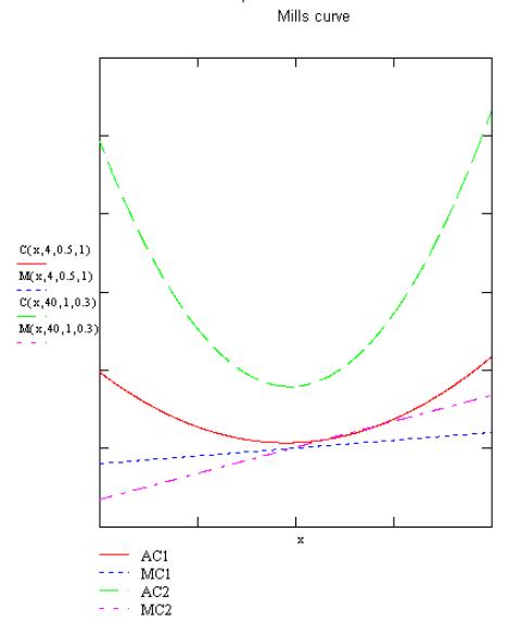
Figure 10. Flexibility and cost curves according to
Mills (1984).
Takala (1994) has proposed a more practical economic analysis, which originates from automation investment justification analysis. Here the measure of flexibility itself is not taken into consideration, but the cost effect in investment. In this analysis, flexibility refers to machines' general ability to cope with variations. When plotting the amount of flexibility on a diagram where the x-axis is the investment (monetary units) an s-shape is derived. First, the flexibility is on the original level – in so called normal conditions. Then by increasing the operating or investing cost a greater ability is achieved. This continues until technological constraints start to decrease the gain. Finally, the amount of flexibility will remain at its maximum. The concepts here are (1) characteristic flexibility referring to the current location on the graph, (2) structural flexibility, which means the direction of change and (3) the maximum level of flexibility – strategic flexibility.
Figure 11.
A case of hypothetical flexibility as an investment curve (Takala 1994).
Gustavsson (1984) suggested the measurement of flexibility in economic terms. His approach considers drastic changes in market demand and an increasing amount of product variety. Flexibility is compared against the perceived or expected uncertainty and economic break-even-point analysis is used for understanding the sensitivity to market changes. In the case of automation investment, money saved in direct work is worth the corresponding investment in the expected life cycle. The theoretical study sees three major types of flexibility: demand, product and machinery flexibility. Consequently, Gustavsson suggests adding capacity in small steps in case of expected demand fluctuations. He also recommends modular design when the risk of fast product changes is possible. In a scenario of technological change, for instance changing the raw material from metal to plastic, outsourcing is recommended (Gustavsson 1984). Although Gustavsson takes into the analysis some advanced concepts, such as life cycle, technological changes and volatile demand, the analysis justifies an automation investment. The case of agility, where uncertainty is taken for granted and as a way to prosper, is not analysed. Gustavsson sees flexibility as a tool for reactive strategies only.
As shown by Gustavsson (1984) uncertainty has a direct link to cost structures. Variable costs allow greater demand flexibility than long term fixed costs. This has an obvious effect on machine investment decisions, but also on utilisation issues as well as process lead time. In addition, the effect of uncertain life cycles should be taken into account in modern production. Hutchinson and Sinha (1989) have combined the concepts of product life cycle and manufacturing flexibility. In their approach, the flexibility is quantified as a net present value (NPV) of a manufacturing line over time. The life cycle of a product has been simplified into three stages: growth, maturity and decline. The parameters in the model include the times for the three phases, T1, T2, T3 and D for maturity demand, which is assumed to be normal distributed with standard deviation of qD. The composition of this approach is practical for those environments, where uncertainty occurs with life cycles, for instance in consumer electronics. (Figure 12)
Figure 12. Flexibility over product life cycle and demand profile (Hutchinson & Sinha 1989).
The reason for the great number of proposed measures lies perhaps in the different origins of the disciplines. Decision sciences have emphasised the issue of flexibility generally and considered the potential of a system as an option. Manufacturing management research has developed taxonomies for classification of the dimensions as well as practical measurement. Economic research has contributed in the area of transferring the flexibility into performance, especially in terms of money.
A great number of different measures have been proposed, but in many cases the aim has been purely research interest for classification or systematisation of structure and hierarchy of flexibility. Practical construction aimed for production control and planning or operative cost accounting have not been proposed. Cost or value based measures illustrate perhaps the dynamics in the most practical way. However, the enabling factors, the drivers of flexibility, may not be so visible. The linkage between non-financial and financial performance measures is very interesting, since flexibility seems to be in many cases affected by investment justification. According to Slack (1983), the difficulties of quantitative flexibility measurement originate mainly from three sources: flexibility is often a potential rather than performance, it is often connected with other measures such as quality, volume, and delivery. It itself has the dimensions of range, cost and time. The structure of flexibility is very important for the agile manufacturing view.
2.2.3 Empirical research on agile manufacturing
Despite the number of proposed measures, empirical measurement of flexibility has begun only quite recently (Upton 1997). Very often, these studies have focused on a specific industry and used describing measures typical for the branch rather than generic flexibility measures. A great part of the literature discussing agility in manufacturing approaches the phenomena theoretically with worked examples. Given examples often originate purely from the literature (Gunasekaran 1998; Burgess 1994) or consultancy type participative research (e.g. Goldman et al. 1995; Kidd 1994). For instance, Burgess (1994) discusses business process redesign as an enabling technology to achieve agility. The transition to new methods is justified by uncertainty in the market. Vastag et al. (1994) consider competitiveness in global business and logistical support for manufacturing agility. The method of this paper is a questionnaire-based survey. The authors conclude that organisational structures play an important role in a firm's ability to adapt to changes.
One of the first empirical papers on agility was "Flexibility Ratios and Manufacturing Strategy", authored by Ettlie and Penner-Hahn (1994). More than 100 managers within 39 plants over the US were interviewed in this study. The results suggested that measures of flexibility such as the number of parts and product families are independent. According to this study, companies invested in flexible manufacturing systems regardless of their strategic emphasis. The study concluded that time ratios of part family changeover are essential drivers for the ability to change. Of interest in this study is the strategic intent. The empirical data includes practitioners from many industries: both users of economies of scope as well as of scale. The reasons for FMS investments are different; while cost leaders are interested in faster changes and additional capacity, economy of scope users benefit from better market sensitivity. Ettlie and Penner-Hahn (1994) discuss flexibility context and conclude, "any theory of flexibility ought to incorporate independent dimensions of capabilities that reduce uncertainty in an organisation controlled by some directional velocity (agility) measure".
Ettlie (1998) studied R&D intensity and its relationships with global manufacturing performance. The survey was performed in 600 durable goods firms from 20 countries. Agility in manufacturing was defined as average percentile improvements in areas of speed of product development, on-time deliveries, customer service, manufacturing lead time, and delivery lead time. Agility improvements were significantly correlated with R&D intensity as hypothised, as well as with computerisation of manufacturing. The agility measure also showed correlation with improvements in market share. The author suggested in discussion in this study that research should focus on the question of how core technologies differ with respect to market response capability (agility).
Collins, Cordon and Julien (1998) tested empirically the rigid flexibility model, proposed originally in Collins and Schmenner (1993). The idea of the model is that flexibility and market responsiveness are achieved by a simplicity of procedures. Simplicity is seen as an enabler for better supplier responsiveness, reductions for setup time and lead times as well as cheaper products. Interestingly, the rigid model origins from Skinner's (1974) focused factory, which has been widely discussed in the literature on manufacturing strategies. However, there are three main differences in the approaches (Collins and Schmenner 1993: 444):
· Focused factory is an introspective method whereas the rigid flexibility model is oriented on customer needs,
· Focused factory metrics are based on four competitive priorities: cost, quality, delivery and flexibility – rigid flexibility assumes responsiveness to be built from design of constantly adapting manufacturing processes.
· Focused strategy is based on trade-offs between priorities whereas the rigid model abandons trade-off limitations.
The empirical test was performed with a survey, which consisted of data from 800 manufacturing units from five European countries. By analysing factors related to inventory management, product cycle times, new product introduction and customer delivery time, the proposed model would be validated. Traditionally flexibility has been understood as a strike-back to focused manufacturing, but the rigid model combines these two. The authors suggested further work for analysing the practical implications of rigid flexibility.
Typical in empirical studies seems to be the use of rather non-exact definitions of agility. Agility is often seen as a synonym for flexibility. As seen in conceptual analysis, one of the main differences is that agility is primarily a business concept that refers to prospering from uncertainty, and flexibility a technical property of a system. Different flexibility measures and dimensions, on the other hand, are enabling factors for this, but not the only factors. Demand level analysis is useful to give an example of uncertainty in manufacturing. Product demand probably has variation. According to a well-known model (see, for instance, Tersine 1985), the demand data can be divided into several factors, namely trend, seasonal variation, variation cycles and random variation (Figure 8). A specific variation may also exist, referring to a specific exceptional behaviour. In this case, agility could be achieved by such flexible production that allows changes in demand level. However, there might also be other enabling factors. Towill & Del Vecchio (1994) applied the filter concept for the supply chain management context.
According to Goldman et al. (1995: 3) agility for a company is being capable of
operating profitability in a competitive environment of continually and
unpredictably changing customer opportunities. They refine the definition (p.
41) as making money in and from a turbulent, intensely competitive business
environment. They emphasise the fact that competition in the agility
environment is based on enriching the customer (Goldman et al. 1995.)
Figure 13. Demand variation has components of trend, season, cycles and random (Tersine 1985).
Harrison (1997) compared production-planning practices between a Western mass producer BMW and a Japanese transplant of Toyota. In this study, the measure was the frequency of scheduled and actual call-off quantities. The comparison was made for four similar parts at a single supplier. The distribution shapes were very different. Japanese plants had a fixed schedule and hence benefited from very accurate production programmes. For instance, the Toyota plan was frozen four months in advance. On the other hand, the Western factory was able to modify schedules frequently and offered greater product variety. Harrison produces evidence for this trade-off. He claims that BMW enjoys lean distribution, but suffers from high inventories. Correspondingly, Toyota has lean manufacturing, but worse distribution. This study gives a hint about the importance of the time-aspect in agility (Harrison 1997.)
Berry and Cooper (1999) analysed manufacturing flexibility in terms of change ability - product mix flexibility. The data collected from four case companies included factors such as output and input variables, production run batch sizes and corresponding cost effects. The paper emphasises that product variety may have adverse cost and margin implications while sales and production strategies are misaligned. Understanding the dynamics of production and cost structures is essential when creating a manufacturing strategy for uncertainty. Production batch size has a vital impact on productivity, which should be taken into account especially when capital costs and utilisation requirements are high.
Suarez et al. (1997) examined relationships between different flexibility types. They examined 31 printed circuit board plants belonging to four manufacturers around the world. Their empirical part was carried out by interviews. The results of this study are some of the very first ones examining the practical effect of flexibility dimensions. This piece of research included factors of volume, mix and new product introduction flexibility. The main findings were:
· The plants with most mix flexibility had the lowest volume fluctuations. This is explained by the buffering effect of a large product variety.
· Mix flexibility and new product flexibility seemed to correlate strongly. This could be due to similar enabling factors, for instance fast setups and high programming flexibility.
The authors concluded also that there is no relationship between mix and flexibility measures, which is assumed also in dimension studies. The study showed slight, but statistically non-significant, correlation between volume flexibility and new product flexibility.
Pagell and Krause (1999) found no relationship between measures of environmental uncertainty and operational flexibility in a survey among North-American manufacturers. They also perceived no significant relationship between performance and a firm's effort to align the level of flexibility with uncertainty. The authors warned against generalising these results, but propose further critical research on the subject. This study provides evidence for the theory that the selection of flexibility measures and corresponding performance measures have a great impact on results. In addition, understanding the relationship between sales and manufacturing strategies is critical. The operational level of measurement is the most important from this viewpoint.
2.3 Production dynamics
In order to understand the possibility of coping with uncertainty, an analysis of production dynamics is also needed. The dynamic behaviour of production makes control extremely difficult. The time delays within the information and material flow are the main parameters here. Delays occur not only in operational manufacturing decisions but at the tactical level too, such as in decisions on capacity additions. System dynamics is a methodology which has succeeded in describing the complexity of manufacturing.
2.3.1 Structural dynamics of response
The order decoupling point stands for the point in the material flowpath where orders are placed and for differentiated products. This points remarkable in that it defines some of the production control characteristics. If an order is released on the final product inventory level, then we are operating on make-to-stock production, and while order releases manufacturing from the raw material level, the production type is make-to-order. Correspondingly, in the intermediate products case we see assembly-to-order. If product manufacturing requires additional design or customisation to a great extent, we could consider an engineering-to-order production. (Bertrand & Wortmann, Wijngaard 1990b)
The order decoupling point should be delayed for greater order fulfilment speed. On the other hand, the decoupling should be advanced for greater product variety and less inventory. Analysing this trade-off is very practical when designing fast response mass customisation systems. Standardised component designs and the use of platforms help to gain better production performance. By introducing uncertainty of orders and increasing product variety, the problem of order decoupling point location becomes more complicated.
Goods flow control
Figure 14.
The order de-coupling point defines the production type (Bertrand et al. 1990b).
Bartezzaghi and Verganti (1995: 158–159) refine order-decoupling point analysis by introducing D:P ratio. The D:P ratio describes the synchronisation of production system – the ratio between own lead time and supplier lead time. Hence, D stands for delivery lead time, in other words the time between order and delivery. P is correspondingly the total or cumulative lead time for a product. This is the time that is required for raw material acquisition, manufacturing, assembly and distribution. Traditionally this P parameter affects the shortest possible forecasting horizon for the master production schedule (MPS) (Burbidge 1994: 102). If the D:P ratio is less than one, purchasing should be made at least partially based on forecasts. Accordingly, when the D:P ratio is more than one, production can run on a customer order basis (Bartezzaghi & Verganti 1995: 158). If the D:P ratio is combined with a degree of certainty of demand, we shall arrive to Bartezzaghi and Verganti's framework for production planning. The degree of certainty stands for qualitative or quantitative knowledge about demand prior to customer orders arriving. While product variety increases, the making of precise production forecasting gets more complex for a single item (Bartezzaghi & Verganti 1995: 158).
Figure 15. Positioning the planning environments according to Bartezzaghi & Verganti (1995: 158).
The assumptions and limitations discussed above do take place in many industries. Even in some traditional mass production (refer to Schonberger's criticism 1990) – for instance, the automotive industry operates nowadays almost without exception by the make-to-order principle. A more typical example of an industry where these assumptions hold, is the electronics industry, where short life cycles, and uncertain short forecasting horizons are taken for granted (Rajagopalan, Singh & Morton 1998). For example, in mobile phone manufacturing, an average life cycle of a product is one year. The laptop computer industry has a life cycle of only six months. In such products with integrated architecture, the life cycle of a product also defines the life cycle of the production line. Increasing uncertainty enhances the need to be prepared for changes and the need for a deeper understanding of the effects of flexibility factors.
2.4 Conclusions
This chapter has dealt with literature and theory related to the problem. First, the existing theory of agility and flexibility was analysed. Then the proposed measurement systems and their linkages to performance were discussed. The literature analysis showed a vast number of proposed frameworks, but on the other hand, also the lack of operational measures. Because of various definitions, the total picture is confusing. The common parameter for the measures seems to be uncertainty. Other factors vary by application and environment. The capability to make a difference between potential, actual and required flexibility is an important property for measures, which are also related to the issue of quantification of flexibility. As summarised in Table 4, there have been mainly two kinds of theoretical work: those describing flexibility dimensions and their hierarchy and those aiming to demonstrate proposed measures. On the other hand, those studies originating from manufacturing strategies literature see flexibility as having economic value for a company. Highly technical measures, mainly originating from studies in mechanical engineering or operations research, perceive flexibility as the property of a system to perform multiple tasks. More recent empirical research, such as Suarez et al. (1997) and Upton (1997) have aimed to combine the knowledge in dimensions as well as practical measures. However, the dynamics between enabling factors and outputs has remained rather unclear, especially in empirical work.
![]() Table 4. Comparison of proposed flexibility
measures (author).
Table 4. Comparison of proposed flexibility
measures (author).
|
|
Dimension identification as Gerwin (1993), Browne
et al. (1984) or Chen et al. (1992) |
Direct technical measure |
Indirect economic measure |
Identification of actual, required and potential
flexibility |
|
Bertrand et al. (1990a) |
Volume and mix flexibility |
Yes |
No |
Yes all |
|
De Groote (1994) |
Mix flexibility |
No |
Yes |
Actual yes, potential/comparison? |
|
Mills (1984) |
Volume flexibility |
No |
Yes |
Yes all |
|
Son & Park (1987) |
Mix flexibility |
No |
Yes |
Actual |
|
Brill & Mandelbaum (1989) |
Machine flexibility |
Yes |
No |
Yes all, but task dependant |
|
Zelenovic (1982) |
Machine flexibility |
Yes |
No |
Actual, others? |
|
Upton (1997) |
Mix range flexibility |
Yes |
No |
Actual - Required. |
|
Bateman, Stockton & Lawrence (1999) |
Mix response flexibility |
Yes |
No |
Actual, potential. |
|
Parker & Wirth (1999) |
Volume |
No |
Yes |
Yes all. |
|
|
Expansion |
No |
Yes |
Required, potential |
|
Hutchinson & Sinha (1989) |
Volume / Product flexibility |
No |
Yes |
Yes all, good quantification |
|
Jordan & Graves (1995) |
Routing flexibility |
Yes |
No |
Actual, others? |
There is a gap in existing research between economic analysis and the enabling factors. Structural analysis has not been combined with empirical measures, which can show the actual level of perceived flexibility as well as the required level and the full potential provided from the system. The dynamics of perceived flexibility, produced outputs and those parameters that have an effect on flexibility or response, have not been demonstrated yet. For this reason, the analysis of the agility concept should be extended to the supply chain context. Based on the literature review, we can conclude that the research we are addressing in this thesis includes the following issues which should be taken into account:
(a) Agile manufacturing and flexibility are polymorphous concepts, none
of the various definitions are widely accepted.
(b) The need for agility originates from market econometrics and the
prioritisation of market performance as well as from uncertainty in these
parameters.
(c) Dynamic behaviour emerges especially in supply chains. This aspect may have connections with agility and flexibility.
This paper seeks insights for combining the agile manufacturing approach suggested in the current literature with dynamic analysis of the supply chain. This will include system dynamics based modelling of a supply chain with constraining capacity. We will analyse the economic consequences in different stages of supply chain. We will also consider policies for guaranteeing product availability level in situations of uncertainty.
3 Agile manufacturing in the electronics industry context
In this chapter, the research environment is introduced. Agility/flexibility issues in the context of the electronics industry are discussed at a general level. Uncertainties and their effects on productions are reviewed. Some managerial choices within the company are discussed and finally the framework for agility and flexibility measurement is introduced.
3.1 Overview: electronics manufacturing environment
The context of this study and examples we use to demonstrate the proposed measurement framework in practice is the electronics industry. For this reason, a brief overview on the electronics manufacturing environment will be given. Typically a production system in electronics consists of three major phases: printed circuit board (PCB) manufacturing, component mounting and soldering; and finally the assembly operations part (Danielsson 1995) (see Figure 16). Between these stages the logistics operations take place. Goods are moved within the manufacturing unit or between factories. The first stage, the printed circuit board part, is batch based manufacturing. The board manufacturer selects the right board type for the application and cuts the boards to the right dimensions. This part of the process is typically done by a company specialising in printed circuit boards only.
The second stage, component manufacturing, often includes highly automated component mounting and soldering. Larger components such as capacitors and transformers are mounted on board by using through-the-hole technique (THT) and soldered, smaller components are very often attached by using surface mounting technology (SMT). Then the boards are shipped to THT/SMT manufacturing, where components are mounted either automatically or manually on the board. After that the boards are soldered and their functionality is tested. Generally, the production phase of component mounting requires high quality control and fast operations for profitability. The last part, assembly operations, is a labour intensive production phase as opposed to the machine intensive PCB manufacturing and mounting. The assembly operation consists of attaching the board on housings, their wiring them, testing and configuring the customer parameters. Sometimes assembly may be divided into two sections, sub-assembly and final assembly. Sub-assembly operations can be performed after component mounting, while final assembly is dependent upon customer modifications. The next step is sub-assembly, where cards are assembled and installed in their containers. The control panels are mounted and wired and linked with the external communication and supply ports. Testing software is installed in the product and the functionality tested. The last phase in the process is final assembly and configuration, which gives the properties for the product as required for the specific application. The final software is installed and configured. Communication ports and peripherals are also installed. The product is labelled and finally tested. The product is packed with equipment and the current language version of user manuals. Despite technological advances, assembly automation is still a new area and rather expensive. With automation high volume is required for achieving a reasonable financial performance and there are still problems with adapting systems with short life cycles and frequent ramp-ups. For this reason, assembly and packaging automation is not very common.
Electronics products consist of physical parts and software parts. These kinds of products are called embedded systems. Quite often products are differentiated from the software part and hardware is used as a platform for a great number of variations. Through the use of software updates, large changes can be implemented without affecting production much or not at all. Use of software as a part of the product is one of the reasons for modern products to be more cost flexible. Modifications are cheaper than in rigid hardware systems, although the high volume production cost may be lower. Because of software the components, electronic manufacturing includes very much various testing. In many cases, test of the product takes the largest part of the total manufacturing time. Hence the product spends its most time in different kinds of testing.
All the production procedures mentioned in our supply chain example can be performed on one site. However, it is very common that only the final assembly and sub-assemblies are made in same production facility. PCB manufacturing is purchased from someone with higher volumes. Also the SMT/THT process may include rather extensive sub-assemblies and testing. Especially with products with modular architecture, for instance industrial electronics, greater technical possibilities may result from outsourcing more extensively. Vertical integration also takes place between manufacturing technologies. Due to the supply chain structure and high delivery performance requirements, product availability concept is important in this context.

Figure
16. Typical
production phases in electronics production process.
(author)
Rapid changes take place in electronics industry. Consequently, uncertainties occur in terms of volume, mix and product life cycles. Manufacturing plants can do relatively little to control the drastic demand changes. The capacity of production needs to be adjusted. Capacity changes derive from changing product sales, which is depending also from the total product variety. Due to this volatile environment, electronics industry has been used in some recent flexibility related studies. For instance, Suarez et al. (1997) based their process range flexibility research on the printed circuit board manufacturing. Berry, Naim and Towill (1995) studied agility of the supply chain in electronics manufacturing context.
Precision of timings is the challenge of modern manufacturing. Products based on new technologies should be placed on the market in early stage and thus the ramp-up time requirements are high. This new technology or product-based competition requires much attention. In addition to traditional sales changes due to global economic trends or seasonal variation, customer segments and technologies should be analysed separately, at least in the first analysis. Managing the risks in a fast changing business is important. Vertical integration presents a solution in electronics. Outsourcing the manufacturing is a typical way to cope with capacity changes. Different companies design the products and technologies than actually make the products. The vertical integration decision is made based on business competencies, but it includes also risk sharing. From customer point of view, this structure helps companies to become more flexible in terms of costs. Contracts are made for a given period of time and for a certain product family or product type. Prices are updated on regular basis, depending on price erosion and the nature of markets, e.g. technological changes. The risk of volatility is decreasing for customers, because in terms of cost accounting, manufacturing has changed from long-term investments to a unit based sales price. At the same time, contract manufacturers enjoy greater volumes and revenues from shared risks.
Customers of electronics contract manufacturers expect precise delivery and co-operation in pricing questions. Consequently, these are very similar compared to the competitive priorities presented in the first chapter. Electronics Business Magazine interviewed fifty electronics business executives who worked with contract manufacturers (Harbert 1997). The survey suggested these manufacturers should reduce lead times, and being more flexible, improve delivery performance. For the distribution service providers, the survey suggests carrying more inventories to reduce supplier's lead times (Harbert 1997). These selected opinions emphasise the importance of lead time reduction and response. Original equipment manufacturers are pressured by the capability of their suppliers. Delivery performance, the availability of items and lead times were considered to be an issue with more than 50% of the respondents. The results of the study describe policies and practices then used in purchasing and co-operation. In addition, suppliers were ranked based on their sale items, purchasing volume, etc. Electronics Business Magazine concluded from the results that the biggest challenges to component manufacturers and distributors are delivery and availability. Improvements in inventories and time-precision were mentioned most often. The second most important factor after delivery was the ability to be competitive in terms of pricing (Figure 17). This survey has not been repeated more recently, but most probably the situation has not changed very much in the meantime and thus justifies the use of this industrial segment within an agile manufacturing framework.
The general presumptions made in the introduction to this thesis seem to be present in the electronics industry. Short life cycles in addition to the aim of precise delivery make the fulfilment of the objectives challenging. "In the dynamic region, product competition is even more complex and volatile. Models can vary, change and die simultaneously. The mixture of different types of model change presents a difficult manufacturing challenge. Design changes can increase variety, or leave it unchanged. In fact, model changes are both the source and the enemy of model variety. This description fits in a growing number of globally competitive manufactured products. Computers, machine tools, automobiles, specialised semiconductors, and medical equipment are just a few of the product categories where the models in product families are exhibiting more dynamic behaviour." (Uzumer & Sanderson 1995: 589)
Figure
17.
Survey of contract manufacturers: Major challenges faced when dealing with
component manufacturers (Harbert 1997).
3.2 Product availability – value and cost of time
The purpose of the product availability approach is to acknowledge the value of fast delivery. As suggested by professional interviews, high delivery performance is an important competitive priority in the markets. In practice, the value of having fast order-fulfilment may emerge via the ability to add sales into new markets and customers. There is also the possibility of obtaining a higher sales price if the lead time is shorter and more consistent than other competitors (Stalk & Hout 1990b). In any case, the value of delivery performance is determined by the customers. The value is assessed against costs, which may depend on capacity utilisation, cost structures and inventory cycles. Figure 18 shows the value and cost of lead time. The example is hypothetical, but it shows the general structure, which is supported by Stalk and Hout’s (1990b) empirical work. Lead time performance increases to the right and in this case the unit cost grows exponentially as a function of lead time. The markets are price-sensitive to lead time also exponentially, so for this production system there is a market to compete in from slowest performance to the crossing-point of costs and price curves.
Figure 18. The value and cost against the lead time (author).
Despite admitting that delivery performance is an important competitive priority for markets, the current cost accounting systems used by companies tend to emphasise the unit cost only as function of production volume. An important trade-off with lead time is not widely used in cost management. Only a few theoretical studies related to economies of lead time have been carried out. The concept of specifying product availability has been proposed earlier to be related to capacity control (Helo 1998a). The key idea is that customers are willing to pay for fast delivery. Production costs also increase when guaranteeing better availability but probably less than the econometric preference curve.
Why is managing the product availability both on the sales and purchasing parts so crucial then? The value of lead time can be illustrated by three main components (see Figure 19):
(a) The direct customer value – customers can benefit from faster delivery, for instance by applying new technology provided by the product. They may also be willing to pay for this advance (Stalk & Hout 1990b). Schmenner (1988) claimed that reducing lead time is the single most important determinant of improved factory productivity.
(b) The cost of lost opportunities – what production cannot supply in time is lost revenue. In Figure 19, this is the area in which the actual production lags from the desired demand (Houlihan 1987.)
(c) The unsold inventory – this negative value component emerges when the produced goods exceed the current demand. The cost of carrying the inventory can present an important share of total costs, especially when price erosion emerges in the market (Houlihan 1987.)
Fast changes in the product and component variety drive the need for good lead time performance. Direct customer value emerges especially when the market would need new technological solutions and can benefit from these. Profits are higher at the beginning of the product life cycle due to better market price. Launching a new microprocessor would be a typical example of this. Frequent design changes make it difficult to manage the inventory well. The reason for this is that short technological life cycles drive price erosion. Having old components in supply may become expensive after a product change in manufacturing. On the other hand, the cost of lost opportunities may be so high in the beginning of product ramp-up that good product availability should be implemented by not considering the inventory cost.
Figure 19. The value of delivery performance (adapted from Houlihan 1987).
Demand changes are only one perspective of the uncertainty perceived by the manufacturers in the supply chain. One of the most challenging issues is uncertainty caused by variables during the forecasting horizon. Even if the trend of sales for a specific product family is known, great fluctuation between product variants often makes the information worthless. This is true especially when the number of product variants is large, because forecasting demand for each type over a short period is very complex. If products are made in a short delivery time based on firm orders, short term variation of volume may be extremely volatile. Also the risks related to keeping finished products in stock are too high, since production life cycles are short and product variation large. The key issue here is the location of the product differentiation point. Reacting to variant changes in short period of a time is easier the later differentiation can be performed. For this reason, products tend to be designed in a way that most of the changes can be made by installing different software versions or changing configurations. In addition to these modification based architectures, modular structures are helpful. Bus, slot or module based standardised interfaces enable greater changes within a product platform. A certain level of component commonality can be achieved from integrated structure by using any of these solutions. Product architecture has an important role in transferring and dampening the demand fluctuations into purchasing orders.
Accurate production forecasts would help in responding to demand changes. However, the forecasting horizon in electronics manufacturing is quite short. According to the contract manufacturer survey "Contract Manufacturing from the Global Perspective 1999" (Gordon and Livingston 1999) there is a pressure for better forecasts.[10] Figures 20 – 22 present some results from this study. This first one illustrates the frequency and accuracy of production forecasts provided by OEMs and the same figure as verified by contract manufacturers (CMs). Figure 23 shows that generally contract manufacturers which are located upstream of the value chain perceive more uncertainty in forecasts than the OEMs. According to the same survey, typical lead times for order-fulfilment vary from 10 to 60 days, while the average is about 30 days (Figure 21). These figures explain that there is a delivery performance pressure upstream of the supply chain. Forecasting information seems to get worse while travelling in the chain. Uncertainty and the need for capability to adjust to new situations are increasing upstream. This study also gives some hints about the capability of reacting to changes. Figure 22 shows the increase of lead time in the case of expanding demand. According this survey a 20% increase in demand may affect about 13 days on average (varying from 4 to 26 extra days). Of course, this parameter is dynamic and depending on the capacity utilisation and current demand level, but it gives some insights into what kinds of variables are measured in the companies.
Figure 20. Frequency and accuracy of production forecasts over forecast horizon used in companies (Gordon & Livingston 1999).
Figure 21. Lead times for manufacturing service companies, including several market sectors in electronics (Gordon & Livingston 1999).
Figure 22. Ability for response in contract manufacturers (20% increase in demand) (Gordon & Livingston 1999).
3.3 Proposed framework for agility and flexibility
A lot of literature deals with making the distinction between those flexibility dimensions that are related to demand, and those which enable the flexibility dimension. For instance, machine flexibility (Browne et al. 1984) could be explained as a result of programming flexibility (Chen et al. 1992). On the other hand, some classifications are very general and do not prioritise the dimensions for the context. Sequencing flexibility is an important issue in many process industries but in electronics manufacturing it is practically applicable to only the single machine context. By taking the electronics manufacturing perspective, we can make some de-limitations. In this paper, we will consider only those uncertainties which originate from the market environment (i.e. external flexibility). The references in the overview suggested that electronics manufacturers’ top priorities are related to product availability and pricing issues. For this reason we will value agility / flexibility against lead time and cost. These attributes are connected to three uncertainty dimensions, which are typical of the context:
· Volume flexibility – the ability to change throughput in terms of response and range,
· Product mix flexibility – the ability to change products in production in terms of response and range.
· Life cycle flexibility – the production ability to change the expected life cycle of a product
For the customers these dimensions are visible properties of agility, the dimensions of externally uncertain market requirements. This definition is compatible with thise earlier presented in the literature (Vokurka & Fliedner 1998, Gunasekaran 1998, Baker 1996) and allows the possibility for us to use the framework of flexibility research. The difference between agility and flexibility is thus time-related. Agility can refer to any flexibility dimension, while flexibility refers either to range or response.
The proposal is for a
hybrid flexibility framework based on a horizontal category refined with
object-based classifications. According to Vokurka and Fliedner (1998: 166)
agility is the capability to react to change in a dimension beyond flexibility.
Flexibility refers to company's ability to adjust from one operation to
another. Agility, however, can refer to any dimension of flexibility. The key
difference according to Vokurka and Fliedner is the ability to react
tonon-predictable changes in markets. Swink and Hegarty (1998: 378) stress the
difference between manufacturing outcomes and manufacturing means. The
definition for general flexibility is proposed as follows. Flexibility is the
ratio between change in the first parameter and corresponding change in the
second parameter. In economic analysis,
the second parameter is cost. Measuring
agility consists of several dimensions, which relate to corresponding
uncertainties (Helo 1998b). Each of these dimensions have two components, these
are:
· Time – the responsiveness aspect stands for fast reaction times in supply chain and production rate;
· Cost dimension – the ability to change cost effectively in terms of volume, mix and life cycle.[11]
The agility of a manufacturing system is considered to be a derivative of these generic dimensions. The practical aspects, used in this model, are volume flexibility, mix flexibility and life cycle flexibility.
3.3.1 Volume flexibility
As proposed in the general flexibility framework, volume flexibility is measured against production costs and lead time. Volume flexibility in terms of cost is the ratio between the change in production volume and change of cost (Equation 3.3). If production volume increases but the cost does not increase as much relatively (or as a percentage), the production system is a flexible one (f > 1). If, however, in the case of increasing production volume the costs increase relatively more, the system is inflexible (f < 1). There is a balanced state when f equals one. In terms of capacity, the important parameter is the load: idle capacity makes f > 1 and full capacity f < 1.
(3.1) 
Correspondingly, volume response flexibility in terms of lead time is a similar equation (3.2). A change in volume affects lead time.
(3.2) 
If the change of production volume is greater than for delivery time, the system is flexible (f > 1). This may be due to slack capacity or good supplier performance. On the other hand, if volume is increasing and delivery time is growing relatively more, the system is inflexible (f < 1). The reason for this can be in lack of capacity or poor supplier delivery performance. Flexibility is always connected to a period of time t. The selection of time period dt should be connected to planning period and always dt¹0.
3.3.2 Mix response flexibility
Analysing mix flexibility has been a research challenge for a while. The definitions have been very different from each other. The main problem has been classifying the flexibility property into that of potential, required, and actual. In order to analyse the problem related to product mix a describing measure is required. For production control and agility, the interest is in the change to response and reactivity. From the literature we know that lot sizing decisions have the most important effect on mix response (e.g. Anderson 1997). The question of mix range flexibility, in other words how the system is capable of manufacturing different potential products and operations, is not operationally applicable because the range issue deals with capital investments, but is very fuzzy since it relies on assumptions of product difference. For this reason, the proposed framework includes analysis only for mix response properties.
Measures for response of mix flexibility are similar to volume measures. Flexibility is here understood to be a ratio between changes of cost and delivery time in proportion to changes of setup. As seen in the literature review, mix flexibility has been confused with some measures describing the product variety. In this thesis, we see flexibility merely as the ability to react to changes. The number of products is more a condition which may create uncertainty in the system and against, which the flexibility should react. Consequently, we use as a describing measure for production mix here the mix ratio, which stands for the ratio between production volume and number of products. This approximation assumes equal consumption for each type of product, which may not be true in practice. However, this measure gives some insight into variability in terms of product mix. In this measure, the values of the ratio becomes bigger when production volume increases or the number of products decreases.
(3.3) 
Similarly the product mix flexibility dimension stands for the capability to change products in production in terms of response and range. Production volume is assumed to be constant and the production mix as a changing parameter. For example, response flexibility could be measured as a percentile extra time caused by gradually increasing variance in the production mix. In addition, mix range flexibility could be measured by analysing product similarity from the manufacturing point of view. Manufacturing time variance would work here. Here we concentrate purely on production control issues and not on discussing the variances in physical dimensions of the product.
Mix response flexibility measure here is the ratio between change of costs and the corresponding change of lot size (b). If the change in cost is increasing more than the change in lot size, the system is cost flexible for mix (f > 1). And f < 1, if the change ratio is vice versa.
(3.4) 
For mix time based mix response, if the length of setup increases but the relative delivery time is does increase, the system is flexible. In the opposite situation, the system is under-flexible (f < 1).
(3.5) 
The response property of mix flexibility depends very much on utilisation. In the case of slack capacity, even long setup procedures cause little in the way of costs. On the other hand, the mix change ability depends also on product architecture and suppliers. If change from one product type to another includes the changes in used components, and the inventory cannot buffer the change enough, the delay in ordering new amounts of components constrains the time based mix response flexibility.
3.3.3 Life cycle flexibility
Life cycle flexibility is a dimension related to production systems' ability to cope with time. A production system with good life cycle flexibility would benefit from good economic performance in changing products. In the case of high life cycle flexibility, the uncertainty in the expected product life cycle would not affect profitability. Life cycle flexibility is the production ability to change the expected life cycle of a product and measured as percentile uncertainty. Practically this dimension is concerned with the speed of ramp up to volume compared to total life cycle of the product. However, the life cycle flexibility is connected not only to new product introduction, but changing to next one as well. For this reason this dimension is related to the cost effective ramp-down.
(3.6) 
Cost terms for the life cycle flexibility are related to sensitivity to change. If the life cycle shortens but the unit costs do not increase proportionally (small product life related fixed costs and fast ramp-up time for production) the system is flexible (f > 1). If the life cycle shortens and the costs rise more (large capital investments or slow ramp-up) the system is inflexible (f < 1). The same behaviour can also be analysed against the average product availability. If the life cycle becomes shorter but the change in average product availability does not go down the system is over-flexible.
(3.7) 
Product life cycles are not only short but also uncertain. Likewise, production, which is based on single production technology, also has a risk component. Taking the effect of uncertainty into account at the operational control level is awkward. When objectives include right timing, early market entrance, right product properties and optimal exit from the markets, uncertainty cannot be neglected.
3.3.4 Technological flexibility
In addition to flexibility of volume, production mix and life cycle, another interesting property is the technological change ability. This property is related perhaps more to product design than production management. However the drivers and enabling factors are very similar. The drivers here are the number of changes or the scale of changes for the product. This change ability can be measured against changing costs as well as delivery time. There are similar rules for the flexibility balance point occurs as for the other dimensions. Thomke (1997) proposes a very similar measure for technological flexibility. Instead of cost, he suggests using profits for the company. Hence, flexibility is defined as the ratio between changes in profit and the number of changes. This example of technological flexibility demonstrates the adaptability of the measure.
In new integrated products, chip manufacturers have a lot of power. Adding customer-focused software to modify the functionality of a product is a way to add value. This has led to situation where manufacturers have to re-consider their place in the value-chain. For instance, U.S. Robotics Inc., a world-known modem manufacturer, changed to Texas Instruments' digital signal processors. In the beginning of the 90's all modems were updated by changing hardware. By using technologically flexible product architecture, new generation products can be updated by downloading a code to the chip (Ristelhueber 1997.)
3.3.5 Agility measurement
Agility is a business level measure similar to flexibility. Whilst flexibility is connected to cost performance in uncertain environments, agility may refer to cost efficiency or the value creating side. According to the definition taken in this paper, the major different between agility and flexibility is the level of concern. We claim that flexibility is always connected to the cost aspect and the concept of agility refers to sensitivity of the productivity of a firm. Agility is a business measure, which is assessed against the productivity of a company, whilst flexibility may be analysed against market parameters such as cost or lead time sensitivity. In other words, the agility of the company is the sensitivity of the productivity, whilst changing the uncertainty parameters of volume, product mix, or product life cycle. Analytically this may be expressed as follows:
(3.8)  and
and  ,
,
where p is the productivity of the firm defined as the ratio between total tangible outputs o and total tangible inputs i. The total productivity of a company in our aspect is the ratio between created outputs, and the used inputs, measured as units of money. This approach makes it easier to compare different creators of value, such as labour, purchases, capital, etc. (see Davis 1955, Craig & Harris 1973).
In addition to the agility definitions mentioned in the literature review, the definition taken in this paper is compatible with Norman and Thisse's (1999), who see agility as a capability that "..allows firms to customize their products to the requirements of heterogeneous consumers at little or no cost penalty." Also the Baker’s (1996) analysis on the differences is rather similar to this operationalisation. Thus, according to our definition, agility may include not only aspects of flexibility related to each dimension, but also issues related to the reconfigurability of a system. In practice this kind of action may refer to more than one flexibility dimension at the same time. The proposed measure for agility may be theoretical and probably it is not very useful actually to calculate a practical value for this, but it connects the measures of flexibility and agility to a larger theoretical framework, namely productivity measurement. In any case, agility as presented is a short-term measure, which is suitable for system comparisons rather than actual systematic and operational performance measure.
The proposed agility/flexibility framework for electronics manufacturing has some points which should be noted. Firstly, a required level of agility depends on the uncertainty perceived from the market environments. There might emerge several different kinds of environments that have different requirements for performance capability. Agility and flexibility are dynamic measure i.e. the value depends from on previous value. (e.g. utilisation and cost in increasing demand). The need for these measures may vary also over time. (Figure 23)
Figure 23. The interrelations between agility, flexibility, response and productivity (author).
A lot of attention has been paid to total productivity measurement as originally defined by Craig and Harris (1973). A lot of modifications of this productivity framework have been suggested. Craig and Harris (1973) argue that their measure shows the company as an entity and furthermore maximises the return of invested capital. However, the issue of flexibility was not considered at all. Richardson and Gordon (1980) claim that companies need to utilise different performance measures at different stages of a product life cycle. In the first stage, the firm maximises the performance by concentrating on innovation, flexibility and responsiveness. In the second stage, a firm operates in a growing capacity. Appropriate measures include capacity utilisation, growth, order backlogs, stock outs and lost sales. In the third phase, cost minimisation is important. Measures such as cost per unit, labour productivities, etc. are in use. Performance measurement framework, suggested by Richardson and Gordon (1980), also claims that as product life cycles decrease the importance shifts from productivity to measures related to innovation and flexibility. If a company is ruled by bare productivity measures, the consequences may be dysfunctional.
Gustavsson (1984) proposed that dependence between flexibility and productivity is partly misleading. He suggested that when flexibility is increasing, the productivity should decrease. This claim is logical at first glance, but inconsistent by definition in a deeper analysis. Instead of productivity, one should analyse the trade-off between efficiency and flexibility. By balancing these, better financial performance, good productivity, can be achieved. For instance, great efficiency may be productive in the short term, but in the case of product changes, the efficiency will be lost if flexibility is low. This kind of situation may occur when inflexible automation cannot cope with model changes. On the other hand, great flexibility is not productive if manufacturing is very repetitive and unchangeable. Too much flexibility, compared to the required flexibility, is non-productive if the cost of additional flexibility is high[12]. The behaviour suggested by Gustavsson may be true in some cases, but it depends on other parameters as well. Capacity utilisation is one of these in addition to flexibility and efficiency. The mechanism of efficiency, flexibility and productivity is described in detail in Figure 24.
Figure 24. Efficiency and flexibility are independent components in productivity (author).
Miller (1984) showed that profitability is the sum of productivity and price recovery. Here productivity is understood in a traditional way: the ratio between outputs and inputs (Craig & Harris 1973). The proposed agility framework is compatible with this thinking as well. Agility can be seen as the capability to make a profit by keeping productivity level high in a changing environment. Volume levels and product mix may fluctuate and life cycles change. The agile company can ensure a good level of profitability in these cases too. Conventional productivity measures have considered the time aspect relatively little or not at all. Properties such as the ability to change or fast adaptation are often overlooked. For instance, production systems with equal score, measured by some traditional productivity indexes, may have differences in lead time or new product introduction. Productivity measures currently used do not encourage using time as a performance metric. Strategically, agile manufacturing is based on economies of scope. Product price is not the most important property for the customer. Agility is related to the markets, where uncertainty is great and timing an important objective. Economies of scope is a strategic choice, which relates the agile manufacturing concept to other close concepts such as mass customisation (Figure 25).
Figure 25. Economic structure of manufacturing costs (Tseng and Jiao 1998: 11).
3.4 Conclusions
The practical measurement issues which
electronics manufacturing companies face
in terms of agility/flexibility are related to product availability and
price competition. This claim is supported by some professional surveys. Global
support required by the OEMs and hardening price competition challenges
contract manufacturers to perform better (Roberts 1998). Some of the choices
managers need to decide are related to trade-offs, such as maintaining an
appropriate product availability under shortening lead times and cost pressure.
Typical managerial choices in the electronics industry include the following
issues, which will be studied in the system dynamics section:
(a) Structural dynamics affecting the supply chain.
Fluctuating volume may be connected to component price-erosion. The managerial
challenge is related to appropriate ordering policies and inventory management
principles. What can one do to improve productivity in volatile demand
conditions? This issue is connected to agility and especially the volume
flexibility issue.
(b) Product variety in a
product line has an effect on average lead time and inventory levels. Does a
large number of products necessarily mean longer order-fulfillment response and
worse cost productivity? This question is connected to mix flexibility.
(c) Analysing the life cycle performance and costs. How does shortening lead times affect the productivity? Fast ramp-ups combined with efficient materials handling is known to be an enabler for a good new product introduction. A financial analysis on this issue is made with different production parameters.
4 System dynamics models of agile production
In this chapter, the proposed hypothetical models for agility implementation are presented. The system dynamics models are based on the theoretical framework discussed in the literature chapters and the research environment. The research procedures of this simulation part include two main steps. Firstly, the modelling part explains the proposed dynamics of agility in manufacturing.
4.1 Justification for the methodology
Dynamic
effects occur when the behaviour of a system changes over time. In the late
1950s, Professor Jay Forrester of the Sloan School of Management at the
Massachusetts Institute of Technology developed the system dynamics method for
this purpose. Since then the method has been used widely in industrial research
as well as urban problems, analysing economic situations and in many other
areas where unstructured information takes place. System dynamics models have proven
their applicability in analysing strategic scenarios as well as simulation of
policies and operations. System dynamics has been defined as "a method of analysing problems in
which time is an important factor, and which involve the study of how the system
can be defended against, or made to benefit from, the shocks which fall upon it
from the outside world." (Coyle 1979 in Coyle 1996: 9). Alternatively,
this can be defined "as a branch of
control theory, which deals with socio-economic systems, and that branch of
Management Science which deals with problems of controllability."
(Coyle 1996: 9).
According to van Ackere, Warren and Larsen (1997: 128) the system dynamics approach is appropriate when a system is known to include, and to be greatly influenced by, critical levels that are known to adjust over time, and when dynamic feedback is known to occur. Another advantage mentioned is the ability to combine different parameters and units within a system. Wu (1994) has compared descriptive, physical, analytical and procedural models (Table 4). System dynamics is located somewhere between the procedural and analytical approach. The models can be constructed from numerical data or by descriptive analysis. The outcomes of the model can be verified as in simulation, against field data. The logic behind the dynamics is also more visible in system dynamics compared to simulation. However, system dynamics may suffer from excessive simplification. Analytically the approach is capable of handling only simple examples. But translating systems into mathematical models is easier than in traditional simulation. This makes it possible to use optimisation techniques as well as other formal tools.
Table 5. A comparison of model type (Wu 1994: 219).
This study takes advantage of one particular system dynamics tool, namely Stella 5.11 by High Performance Systems Inc.[13] The Stella simulation software package was used in order to construct the system dynamics relationship among the selected processes. Stella software and the system dynamics approach have been used widely in similar studies, for example: Anderson, Fine and Parker (1996) used system dynamics in their supply chain research. There seems to be a number of established users and a growing interest in wider applications. For a more comprehensive overview of the simulation package and system dynamics methodology generally, see Senge (1991), Morecroft (1992), Checkland (1999), Davis & O'Donnell (1997) or refer to Stella manuals Peterson (1992), Peterson & Richmond (1997). Additionally, the approach used in this study can be classified as an engineering approach for performance enhancement of systems (Pritsker 1997). The aim of the study is to model perceptions from the real world, then make it formalised in a system dynamics simulation model, run the model, visualise the results and compare the outcomes with reality (Figure 26). Managerial suggestions can be made based on knowledge of the model.
Figure 26. Updated engineering approach for performance enhancement of systems (Pritsker 1997: 779).
Many companies do measure non-financial measures and recognize their importance. However, the problem with these is that such performance measures have not been connected and integrated to financial measures (Davis & O'Donnell 1997). The system dynamics approach makes it possible to introduce technical measures, measures describing organisational behaviour, ordering policies, and financial measures into very same model and to quantify these. We can base the justification for use of the systems thinking methodology in this piece of research on three main issues:
(a) The area of agile manufacturing involves a broad perspective, which includes market elements, production and logistic issues as well as cost engineering points of view.
(b) Production dynamics involves feedback structures and delays caused by response.
(c) The behaviour of a production system in various circumstances may be demonstrated analytically.
These three nodes of justification are connected to the strengths of the system dynamics approach. System dynamics is a holistic approach capable of handling complex systems which are involved with feedbacks and delays (van Ackere, Warren and Larsen 1997).
This chapter includes six different simulation models which deal with different dimensions of uncertainty. The reason for constructing several different models instead of one single general model is to demonstrate the dynamics behind each phenomenon in a simple way. Mixing continuous demand models, such as “Forrester Effect” and “Capacity and Dynamics Growth” with interruptive models such as “Mix Flexibility” would result a very complicated and a large model. On the other hand, testing the validity of the model is easier when the number of parameters is low.
4.2 Structural dynamics: demand magnification and order variations
The first tested model deals with the structural dynamics of a supply chain. In the "Forrester Effect" model we will test the agility of a chain with different ordering mechanisms. The knowledge of the analysed behaviour is not new. Since the late 1950's it has been known that internal structures used in multi-echelon systems may create oscillations in demand (Forrester 1958). Forrester's Effect refers to this phenomenon, where the demand signal is amplified from echelon to echelon as orders go through the supply chain. The effect is emphasised especially in longer supply chains and companies operating in the deep upstream - for instance, raw material suppliers. The Forrester Effect is known also as the bullwhip effect - this term refers to the similarity between the graphical behaviour of demand and the cracking of a whip. In some industrial sectors, concepts of whiplash effect and whipsaw effect are used (Lee, Padmanabhan & Whang 1997a: 93), but they are just new names for demand amplification as identified by Jay Forrester.
To illustrate the behaviour of such a system, consider a Stella model of a three-echelon supply chain consisting of wholesale inventory, distribution centre, and a production plant. Between each inventory, there is a delay caused by transportation and order handling (Figure 27). Each echelon operates individually based on demand information gained downstream. This situation describes Forrester's famous "Beer Game" model, where a brewery and distribution centre tries to cope with demand change in the wholesale. Ordering policy has an essential effect on system behaviour. In this model, we use a simple policy which uses weekly sales of markets. In addition to weekly sales from the next phase, the ordering policy for an echelon takes the target inventory and the distribution stock level into account. Target inventory level is considered to be constant for sake of simplicity. The time delay in transportation is set to be 2 between every echelon. The ordering policy taking the delay into account is in the complete form as follows: Orders1 = Weekly_sales+(target_inventory-(Distribution_stock))/correction delay. The correction_delay is a parameter which tells how fast the system should respond to changes. Operationally, it refers to the percentage of difference between actual inventory and target inventory which will be handled within a time unit. For instance parameter value 2 means that it takes two time units to fill the inventory difference. Correspondingly, the next echelon’s orders operate with the same principle: Orders_2 = Despatch_1+(target_inventory-(Wholesale_stock))/ correction _delay, and Orders_3 = Despatch_2+ (target_inventory-(Factory_stock))/ correction _delay. See Figure 27 and refer to Appendix 3 for technical details of the model.
Figure 27. Forrester Effect simulation in a three-echelon supply chain (reconstructed from Forrester 1958).
In this model, the demand for product is stable at 10 units per time for 60 time units. Then suddenly the demand increases to 20 units. As seen in Figure 2 the system starts to oscillate and it takes about 100 time units until the system has stabilised into a new equilibrium. Trace 1 refers to the inventory level in distribution, Trace 2 to wholesale and Trace 3 is the production plant. As seen in the Figure 28, the demand fluctuation amplifies from echelon to echelon in the order stream.
Figure 28. Demand amplification in the supply chain occurs from echelon to echelon, and emerges in particular when demand is changing (author).
The demand magnification effect has been observed both empirically and in practice. To take some more examples, Anderson, Fine and Parker (1996) have investigated the machine tool industry in the US and found the demand variation of this branch, which depends greatly on the automotive industry, being derived directly from the variation of car sales. When gross national product varies by 2 %, the car sales will follow with a fluctuation of 13%, the machine industry with 22% respectively and the orders to suppliers by 37% (Anderson et al. 1996: 5). Similarly, supply chain variation effects have been identified in electronics EMS manufacturing (Lee et al. 1997a: 93) and retail sales (Lee et al. 1997b: 546; Mahoneer & Cheddad 1998; Holmström 1999).
There are a number of reasons as well as possible control parameters behind the effect. Unpredicted changes inflict shortages, which lead to over-ordering as a corrective action. Greater order sizes cause not only uncertain deliveries, but also more uncertainty in demand for the item. Consequently, safety stocks will increase and many lot sizing decisions, such as EOQ, result in greater changes in order quantities. The same loop also works in the case of decreasing customer demand. The signal will amplify (see Figure 3). Based on this perception, Burbidge created the Law of Industrial Dynamics, "If demand for products is transmitted along a series of inventories using stock control ordering, then the demand variation will increase with each transfer" (Towill 1991: 198).
Figure 29. Some general causes of demand amplification (Houlihan 1987).
Towill’s research group has developed the Material Flow Principles based on comprehensive simulations and empirical work in real-world supply chains. According to this framework, the four principles are as follows (Towill & McCullen 1999):
(1) Control Systems Principle refers to the selection of Decision Support Systems, which control the chain.
(2) Time Compression Principle refers the effect of cutting down material and information flow lead-times.
(3) Information Transparency Principle involves sharing the information within the actors of the chain.
(4) Echelon Elimination Principle refers to eliminating echelons from the supply chain, which should reduce the time delays and information distortion.
According
to generally prevailing opinion, the main factors behind demand fluctuations
are the following four parameters (Lee et
al. 1997): (1) demand forecast updating; (2) order batching, (3) price
fluctuation, and (4) rationing and shortage group. One of the most important
factors is information updating in the supply chain. Although it is impossible
to avoid delays in the material flow, the information flow of demand forecasts
should be as smooth as possible. Changes at the beginning of the flow should be
updated to the whole chain frequently, in order to be reactive to change. Order
sizes should not be optimised by dynamic lot sizing models that consider
production plant transportation only. The supply chain should be designed as an
entity with internal delays. For example, consider a situation where a company
is ordering items from a supplier on a monthly basis. The supplier observes
great variation in demand, because in the beginning of the month there are no
orders, but in the end of the month, a large order is placed. This all happens
under the assumption of a smooth demand downstream. Demand fluctuation is
greater from a supplier perspective than from a manufacturer point of view. The
conclusion is that periodic ordering policy increases variability (Lee et
al. 1997b: 97–98.)
Many
pricing policies encourage ordering in larger lot sizes, which definitely
affects the market behaviour. The demand volatility expands and the wavelength
of the signal gets longer. For instance, year-based contracts on total capacity
combined with small transportation lots would help to get out of the
situation. Rationing and shortage
gaming take place when market reactions tend to buffer purchasing, for instance
before large increases in general demand or prices. When customer demand
increases temporarily, over-buying starts in order to buffer with inventories.
The electronics industry is familiar with this situation, especially when using
high technology components that are hard to replace. Companies buy more than
they need if there is concern about supplier reliability. This has been
reported to have happened with RAM chips and with some microprocessors (Lee
et al. 1997b: 97–98.)
Ordering systems are either multiple or single cycle systems. With multi-cycle ordering, components are ordered in different time intervals and lot sizes. Multi-cycle ordering is the most common approach in industry, mostly due to the popularity of MRP-II and economic-order-quantity (EOQ). Despite the good properties of multi-cycle ordering, there is an undesirable effect causing variation in inventory levels and capacity load. When different order intervals occur on a single machine capacity or inventory, there will be peaks in demand caused by orders in the same phase. This phenomenon is called the "Surge Effect" (Burbidge 1996a: 152). In order to illustrate the situation, consider a Stella model, where four different order cycles with the same total volume and a constant demand emerge. The total demand for each time unit is 8 and the ordering system is supplying (a) 10 units per each 5 time units, (b) 20 units per each 10 time units, (c) 40 units per each 20 units, and finally (d) 5 units per each 2.5 time units. Each order utilisation group has an initial value (INIT Capacity_3 = 10), the orders are released in their lot-sizes by using pulse function (Orders_3 = PULSE(40,20,20)). The production rate is similar and constant in each group (Usage_3 = 2). The utilisation is a stock between two flows: orders and production rate (Capacity_4(t) = Capacity_4(t - dt) + (Orders_4 - Usage_4) * dt). See Figure 30 for model details and Appendix 4 for a complete source code.
Figure 30. The Surge Effect model includes four order cycles and a stable consumption (author).
Running the simulation shows very quickly this internally caused variation amplification. A short run shows the average inventory level to be about 37 and standard deviation 18 (Figure 31). The phase of orders is not a adjusted at all and for this reason all orders have a common peak. However, this example gives some insight into how the lot sizes affect the total order level. As stated in Burbidge's Ordering cycle law, "If various components are made in a factory and made at different time cycles, they will generate high amplitude and unpredictable variations in both stocks and load" (Towill 1997: 627). Multi-cycle orders increase the total variability in capacity or inventory, even when stable consumption emerges.
Figure 31. Simulation results of the Surge Effect (author).
In terms of reactivity and predictability, big order batches with long lead times are the most problematic, since adjusting an order to a new level should be done far more in advance than in the case of small batches. This has been noted by Burbidge (1961: 780), who concludes that "the 'flexibility' of a material flow, or its ability to follow demand fluctuation, again depends on batch quantity, frequency and phase." With single cycle ordering systems items are ordered on given due dates and in similar periods. There are not so many such systems in use, even if adjusting a periodic order interval in modern MPC software is not so difficult. One such method is Period Batch Control (PBC), which is basically a control system for Group Technology based cellular manufacturing. PBC was originally developed by Burbidge (1996b), and it is estimated that less than 10% of manufacturing companies use this kind of ordering policy (Burbidge 1996b). In the case of long order lead times, this may be inflexible, but according to Burbidge (1996a: 154) very controllable. In capacity control the surge effect especially should be considered. Costly fluctuations in the load level can be avoided by controlling the whole supply chain instead of one echelon (Helo 1999a; Helo 1999b; Helo 2000; Berry et al. 1995).
With regard to the flexibility perspective, the behaviour related to order magnification and order level variance suggests that upstream companies may suffer from higher volume volatility. This may cause longer lead times for orders and higher unit costs during peak times. Based on these two models, we can propose that the challenge of agility / flexibility is greater upstream in supply chains, because the structural chain dynamic increases the variation there.
4.2.1 Capacity constraining the system – a flexibility perspective
But how does the volume volatility affect the agility / flexibility situation? In order to demonstrate this we will introduce another model which analyses this issue in detail. The manufacturing system concerned in this simulation model consists of an adjustable capacity, inventory and a component supplier. This two-echelon supply chain manufactures multiple products by using make-to-order or assembly-to-order production policies. An order mechanism controls the purchasing and the adjustment system controls the production rate and used capacity.
Sales orders accumulate into a backlog depending on volume. The ratio between orders backlog and capacity defines the average lead time for customer order-fulfilment. Orders variety parameter use setups and consume capacity. High capacity utilisation leads to cost-efficiency. On the other hand, high utilisation makes queue time longer for an order. Cost efficiency and fast delivery are trade-off performances, which cannot be maximised at the same time. Economic reactivity depends very much on the cost structure of the product to be manufactured. In addition to volume, the same order-fulfilment dynamics applies also in the product mix. In terms of mix response, lot sizing decisions have the most important effect on order-fulfilment. Orders variety parameter or smaller production runs, i.e. smaller lot sizes, increase the setup-time, which consumes the available capacity. Less capacity directly weakens the delivery performance. However, the issue of capacity utilisation plays a crucial role in this structure. If the order-backlog stays at a low level and stable, or in other words the ratio between orders and capacity is low, the lost capacity due to changes does worsen the delivery time remarkably. The issue of orders variety will be discussed in sub-chapter 4.3 “Product variety: mix uncertainty and lot-sizing”.
Figure 32. Trade-off between delivery performance and cost efficiency (author).
In the "Agile Production” model the sales are accumulated into an order backlog. This starts production and gives impulses for purchasing. Finished items are released from stock: "Finished_items_stock(t) = Finished_items_stock(t - dt) + (manufacturing_delay - Despatches) * dt". However, the capacity of the production system constrains the despatching equation "Despatches = MIN(Order_backlog,utilised_capacity)". The delay caused from manufacturing lead time is derived as well from utilisation: "manufacturing_delay= delay(shipped_by_supplier,1/utilised_capacity)". The purchasing activity from the supplier is organised from actual sales demand. The ordering policy is based on current sales as: orders = demand + inventory_correction + (target_on_order - Supplier_backlog) / correction_delay. This equation has variable inventory_correction, which takes work-in-process and goods in transportation into account as (target_on_order - WIP) / correction_delay. Targeting is based on assumed lead time from supplier target_on_order = demand * supplier_leadtimeinfo. This ordering policy takes all phases of physical transportation into account and moreover, its reactivity is adjustable with term correction_delay. This parameter defines the sensitivity to changes in finished product demand. The smaller correction delay we set, the more sensitive target adjustment we perceive.
The ability to respond to changes is built on two main levels: These are (1) the local capacity and (2) the supplier system ability. Purchasing activity represents the supplier performance of the chain. The local ability is built into component stock level and manufacturing capacity. The complete model structure from production / operations part is illustrated in Figure 33. This includes order-backlog mechanism at the top, purchasing policy at middle-right, capacity adjustment at middle-left, and the actual goods flow at bottom.
Figure 33. Production and supply part from the simulation model (author).
The dynamic behaviour of production emerges due to delays in ramp-up, delays in logistics and the effects of inventories. Figure 34 illustrates the demand, actual shipments, component stock level, and order-backlog. In the beginning, the ramp-up constrains the production flow. At t=7, the full capacity is in use and the lead time starts to decrease. It is easier to react against the next sales demand peak at time 16, when the system has stabilised at the normal capacity performance level.
Figure 34. Demand, despatch and inventory (author).
Cost structure is a separate section of the model described in the "cost structure" window. Cost drivers, such as despatch, inventory levels or capacity utilisation are located in the actual model and are linked to the financial performance analysis part. Those drivers actually locating in the production part are visible as dotted objects in Figure 35. The financial analysis parties are based on two main cost components: materials costs and fixed costs. The materials costs consist of direct materials consumed and the price erosion component, which increases the costs of components based on the inventory delay (Figure 35).
Figure 35. Financial performance section of the model (author).
The lead time for orders is approximated as a
division between order backlog and the total capacity. The inventory cycle time
is calculated in a similar way: the Component_stock level is divided by
the current level of Despatches. (Figure 36)
Figure 36. Lead time mechanism (author).
In order to analyse the agility in fluctuating demand, we test the model by using demand 3*sin(time)+4. Figure 37 illustrates two cost structure scenarios. The upper part of the picture refers to accumulated productivity in the case of fixed cost structure (90% of costs fixed, 10% variable). The productivity will decrease about 19% in this uncertainty l. the agility of this system is:
(4.1) ![]() ,
,
The lower part of the figure shows the productivity behaviour of a variable cost structure (90% variable costs, 10% fixed) in a similar environment. The productivity is less sensitive to fluctuations, and thus the agility is higher:
(4.2) ![]()
The
analysis of the "Agile Production" model suggests that the
cost structure of a company has an important effect on the firm's capability to
tolerate productively against volume fluctuations. A high amount of direct
materials makes cost structure less sensitive to demand changes. Based on this
we can propose that variable cost structure and low inventory holding costs
enable agility.
4.3 Product variety: mix uncertainty and lot-sizing
Mix response flexibility deals with the issue of the cost of variety. A production system is more flexible the more it can tolerate different products. This discussion can easily lead to assessment of diversity – how different are the products? In our model, we simplify the aspect of only those products, which are already manufactured with the system concerned. Potential new products are not taken into the analysis of flexibility. Lot-sizing decisions both in manufacturing and purchasing have an important effect on lead time. The mix response ability is connected to the "batch and queue" effect (see Burbidge 1961). When utilising a discrete manufacturing system, there is always a concern of appropriate cost efficiency, which is greatly affected by setup costs and lot-sizes.
Figure 37. Productivity
with 90–10 and 10–90 cost structures (author).
4.3.1 Lead time performance and queuing theory
Response is an important performance for a
contemporary electronics manufacturing plant. High product mix and short life
cycles make it difficult to control production by using inventories. Other
methods related to capacity control, setup improvements, and lead time
reduction are needed. Queue models have been used in the literature to analyse
practical applications of production and distribution systems. According to
Karmarkar's (1987) approximation, later modified by Suri (1998), the total
processing time for an individual order is a function of arrival and service
rates, their corresponding variations and batch sizes. These models illustrate
the trade-off between capacity utilisation and lead time well.
Any queuing system can be characterised using a standard shorthand form, A/S/m/N/K/Z, known as Kendall's notation. A refers to interarrival-time distribution, S the service-time distribution, m the number of parallel identical machines, N the restriction on system capacity or the maximum number of jobs, K the size of the external source or calling population, and Z the scheduling rule (if default FCFS, this parameter is omitted). The typical distributions are labelled as follows:-
· M Exponential (Markovian) distribution
· D Deterministic (constant time)
· Ek (Erlang type k (k=1,2,…)
· Hk Hyper-exponential distribution of order k (k=1,2…)
· G General (an arbitrarily specified function)
· GI General and independently distributed inter-arrival times
When analysing the total time of a job in a system, we should consider the total system time as a sum of manufacturing time t and queuing time. Queuing time is a function of l arrival rate for orders, and m, service rate for orders (equal to 1/t). Utilisation parameter r is a ratio between l and m. When assuming negative exponential distribution, caused by a Poisson process of arrivals (random) which take place in many cases, we get:
(4.3) 
In case we are also interested in the effects of deviation of arrival rate (ca) and service rate (cs) we can use the GI/G/1 approximation (suggested, for instance, by Kuehn 1979, Whitt 1983, Shanthikumar & Buzacott 1980):
(4.4) 
This expression is exact for the M/M/1 and M/G/1 type queue systems. In Figure 38, the reader can see the effect of deviation (M/M/1) in function W, and the Poisson process in function W1.
Figure 38. System
time as function of utilisation (arrival rate / service rate) (t=1) (author).
Because of the non-linear nature of waiting time, higher utilisation causes a very long total queuing time. The trade-off between the lead time and queue theoretical utilisation rate shows that all unused capacity is not unproductive. In order to assure product availability, some of the maximum capacity should be idle. The question is how to convert the queue utilisation rate to normal manufacturing utilisation.
Based on this queue-theoretical analysis we can conclude that a certain amount of capacity should be available for the production system in order to keep the lead time within tolerable limits. Practically this means that the system should have idle capacity in terms of utilisation in order to be able to react within the capacity flexibility range. Batch size has a very important effect on the reaction speed of a production line and capacity (Matupi 1997). Lot sizing decisions also relate strongly to the trade-off between utilisation and lead times. However, the concept of batch quantity or size can sometimes be very confusing. It may refer at least to four different batch sizes in manufacturing. These are according to Burbidge (1996b: 16): (1) the order quantity, (2) run quantity, (3) setup quantity, and (4) transfer quantity. These all are individual parameters which may have an effect on the properties of a complete system.
To illustrate the effect of lot sizing and capacity utilisation on the production lead time, we take an example from queuing theory. Assume a M/M/1 system, which uses batching a single product. The lot size is q and u is the utilisation parameter. According to Karmarkar (1987) we can define the waiting time as an equation (2.13).
(4.5) 
In Figure 39, the waiting time is plotted as a function of lot size, which is increasing on the x-axis. There are time curves for utilisation parameters of 0.4, 0.2 and 0.8, which also gives the idea of the behaviour in the cases of different demand levels.
Figure 39. Effects of lot sizing decision on lead time with the utilisation parameters of 0.4, 0.2 and 0.8 (author).
In addition to lot sizing issues, another important issue is the number of machines. How does the number of machines affect the total system time? This can be analysed with the help of queuing theory. By using the equation 2.10 the total system time is described as a function of arrival rate, service rate and number of machines (Tersine 1985). This formula gives the exact answer in case of a M/M/N system, but it can be used as an approximation in many other systems too.
(4.6)
 ,
,
where M is the number of service channels and n a counter.
To test the approximation, assume a machine where m = 5, and changing arrival rate from one to five, with one-steps. Additionally, the same situation is analysed with multiple machines, of which total capacity equals as much as the original one machine capacity. The number of machines M is changed from 1 to 5. Arrival time is changed between 100 and 190 with five steps, and the total service rate is 200. The results are illustrated in Figure 40. The z-axis shows the total system time in different cases, the y-axis is the arrival rates and x-axis the change in the number of machines M. (Appendix 2.)
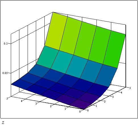
Figure
40.
System time as a function of service rate, arrival rate and number of machines
(author).
4.3.2 Lot-sizing
The concept of batch quantity or size can sometimes be very confusing. It may refer at least to four different batch sizes in manufacturing. These are, according to Burbidge (1996a: 16): (1) order quantity, (2) run quantity, (3) setup quantity, and (4) transfer quantity. These all are individual parameters, which may have an effect on the properties of the system. In order to model the mix response, a "Mix Flexibility" model was built (Appendix 7). This model analyses the response (lead time) of a production system based on queuing theory and Suri’s model (1998: 158 - ). Suri's model originates theoretically from Karmarkar's approximation. The main difference is that Suri's approach includes parameters related to deviation of service and arrival rates, as well as the effect of setup time. The components of average lead time LT (time from arrival of job to its completion) include the utilisation term M, the variability parameter V, and processing time TJ. When all put together we can expand the components into the function of following form of average lead time to process the order: Lead_time = 0.5 * Variation_parameter * Magnification + Batch_processing_time, where
(1) Batch_processing_time = TSU+L*TJ1 and Magnification = Utilisation/(1-Utilisation, Utilisation = ((TSU+L*TJ1)/(L*TA1)
(2) Variation_parameter = ((SJ^2)/ Batch_processing_time^2))
+((SA^2)/((L*H/D)^2)).
The cost part is modelled as follows:
totcost = (fixcost+varcost*units_produced)/units_produced units_produced = L/Lead_time.
The parameter TJ refers to the mean time to process a job (including setup time and process time for all pieces in the lot), The parameter SJ is the standard deviation of time to process a job, correspondingly TA is the mean time between arrivals of jobs to the work centre and SA is the standard deviation of time between arrivals of jobs to the work centre. L is the manufacturing lot size.
The mix flexibility was tested by giving an example with two cost structures in the case of increasing variation (SA). The results are illustrated in figures 41–44. From the results of this model we can conclude that the delivery time in a make-to-order environment is connected to lot-sizes. The smaller lot-sizes in production, the better response speed for different product types (Figure 41). The drivers for cost efficient variety are: Inventory level, Lot-size of manufacturing, Low fixed capital, Utilisation and Setup costs. According to this model, the standard deviation of inter-arrival time increases the lead time exponentially (Figure 43). In terms of global response ability, the issue related to mix uncertainty is connected to part commonality. In the case of high part commonality, a wide fluctuation in product mix will not affect the purchasing operations. On the other hand, a good part commonality should dampen the volume fluctuation due to mix changes.
As the mix flexibility model shows, the lead time issue is connected to lot-sizes and the capacity utilisation. Capital intensive production needs a more stabile demand for cost efficient flexibility (Figure 42 and Figure 44). Labour and material intensive plants can tolerate more changes. On the other hand, if supplier performance is very poor, hence more inventory is required, and at the same time price erosion would emerge, and this would affect the costs as well. Cost effective setups enable shorter production lot-sizes and increase mix flexibility.
Figure 41. Lead time as a function of lot size (author).
Figure 42. Unit cost as a function of lot sizes (author).
Figure 43. Standard deviation of inter-arrival rate vs. lead time (author).
Figure 44. Standard deviation of inter-arrival rate vs. unit cost (author).
4.3.3 Product availability and dedicated capacity
Analytically, the cost of product availability during a time period from t0 to t1 can be approximated as follows. U(x) is a time stationary probability function of the assumed level of production volume x, where m is the mean and s standard deviation for the measure x.
(4.7) 
Correspondingly, A(x) is the effect of production volume x to costs. In this case we consider A(x) as the unit cost for each level of production volume. The risk may now be approximated as a multiplication of these two components:
(4.8) ![]()
The risk may be divided into two the components: The customer and supplier part. Customer part is the area from 0 to x1
(4.9)  ;
;
and correspondingly the supplier risk the part from x1 to the end:
(4.10) 
Setting the risk proportion x1 between customer and supplier risk is a competition question. How much of the risk is taken by the company and how much is included into the cost of availability depends on the market situation. The flexibility dimensions of mix and life cycle can be modelled in a similar way. Figure 45 illustrates the volume flexibility of a production system as unit costs, volume uncertainty as the probability of volume (density function); and the risk as the area of multiplication between these two parameters.
Figure 45. Analytical structure of volume flexibility (author).
One solution for the problem of guaranteeing product availability in an uncertain environment is dedicated capacity for defined availability groups. This means that different capacities are dedicated to certain types of products. In practice, a factory can implement this either by making production lines for customer or product groups or by sharing the capacity time. If production volume is low and volatile, a good solution could be taking a time period of each day and reserving it for certain products. Each product group now has a dedicated capacity and specifying product availability is easy. Especially if production lots have the same sizes in terms of total processing time, the approximated order-fulfilment time is equal to processing time for a lot multiplied by the number of orders in backlog.
In the case of high volume products with different availability requirements, a company can do the capacity dedication by different availability groups. For instance, one hour of each eight hour shift can be dedicated to first priority orders, say one day delivery. The second availability group (lead time five days) can reserve three hours every day. Orders of longer lead time can use up the rest of the capacity. Since each availability group has a dedicated share of total capacity, dividing the costs of capacity is a straightforward procedure. The overtime costs can be divided in the same way. Higher availability groups are costly. Figure 46 shows an example of three product availability groups in a single capacity. The top structure presents the highest priority orders, the middle-one the second group and finally, the bottom parts of the model, the lowest priority orders. Each group has a dedicated capacity and if one group’s capacity is not fully utilized, another group can take advantage from the idle capacity. Full model details are attached in Appendix 7. "Dedicated capacity". Figure 47 illustrates how lead times for production develops in each availability group in the case of a growing order-base. The lead time for Queue 1 as the highest availability group will never exceed the guaranteed delivery time.
Figure 46. Structure for dividing capacity into availability groups (author).
Figure 47. Lead times for three availability groups (author).
4.4 Analysing the product life cycles
The financial performance of a contemporary company depends much on its ability to introduce new products and apply new technologies. The life cycles of many products have decreased in many industries, which forces companies to seek more efficient ways to make applications for new and existing markets. For instance, electronics, telecommunications and software industries are highly dependent on product development performance. However, the measurement of product life cycle related effects in production is difficult. The relationship between productivity and innovations has been discussed widely. Von Braun (1990, 1991) claims that shortening product life cycles leads to a surge in overall company sales, but over time the sales will decrease rapidly to a level which would not occur in the case of longer product life cycles. Von Braun (1990) has demonstrated by using simulation that shorter life cycles reduce the total sales compared to longer ones. Frequent short life cycles also increase the risk to successful new product introduction.
In this paper we concentrate only on a single life cycle level and avoid the dynamics caused by variation in average life. We will use the "Agile Production" model and consider the learning effect which is directly linked to production. For modelling the new product introduction, the model uses a logistic curve as a learning curve, which is an s-shaped growth curve. This is a cumulative version of the traditional logarithmic curve. In the model, the production rate, Capacity, is defined based on the CapStock variable, which is the learning component. This module consists of CapStock, which is controlled by inflow and outflow (Figure 48). The compounding fraction accelerates the learning, whilst the loss fraction starts to reduce the growth until the desired volume comes closer.
Figure 48. Mechanism of s-shaped learning curve in new product introduction (author).
There are many other possibilities to model this behaviour but this option is selected because it is a widely used infrastructure in system dynamics (Richmond & Petersson 1997). This structure yields an s-shaped growth curve, which has three major issues: the starting level (of the production rate), the target level and the time to ramp-up to full volume (Figure 49). In addition to the start-up, the ability to maintain productivity depends also on the ability to slow-down effectively. If the slow-down is drastic, also old components in the inventory are expensive to get rid of. Here the inventory cycle time becomes important.[14]
Figure
49. S-shaped
learning curve in new product introduction
(author).
Product life is related mainly to cost structure, inventory cycle time and new product ramp-up. If production is very capital intensive, the low utilisation due to new product introduction is expensive. The learning curve effect also takes place in the beginning. In the case of short life cycle, the fast ramp-up to full volume is critical. It is quite obvious that the cost efficiency gets better over time, but from a business perspective, there is another priority as well. As suggested previously, the lead time for order-fulfilment may be valuable from a market perspective. The lead times are high in the beginning until the production can reach further up the learning curve (Figure 50 - Trace 5).
Figure 50. Ramp-up to volume and lead time for order fulfilment (author).
An optimal or sensible addition to capacity in growing markets is a problem related to life cycle and capacity issue. Forrester (1968) modelled this problem with system dynamics in the article "Market Growth as Influenced by Capital Investment". The basic idea in the model is in three loops: 1) increasing numbers of orders adds to the number of salesmen, which causes an increasing sales force and more orders; 2) increasing order backlog makes the delivery time slower and decreases sales effectiveness; 3) increasing delivery delay triggers production capacity ordering (Figure 51). The ordering policy for capacity is a discrete logical function, which compares the average lead time to trigger value. If the trigger value is exceeded, new capacity will be ordered (time delay involved between order and installation).
orders_for_capacity = IF((Order_backlog/(Capacity + Capacity_coming_on_line))>delivery_time_trigger) then Capacity_addition else 0
All other functions used in the model are continuous.
Figure 51. The capacity addition process in a case of expanding sales and markets (reconstructed from Forrester 1968).
As a result this yields exponential growth limited only by the rate of capacity additions (see Figure 52). Expansion flexibility (Chen et al. 1992; Suarez et al. 1997), the ability to easily add capability and capacity in a production system, is a related concept here. Moreover, if production rate modifications can be made without changing the manufacturing facilities, we can talk about capacity flexibility (Hernandéz & Vollmer 1998). The flexibility of capacity is the ability to change capacity load, this operates on a master production schedule level and thus includes manpower and machinery. Capacity has an obvious effect on order backlog and delivery lead time. If the market is very lead time sensitive, the optimal addition of capacity is a crucial issue, in the same way as utilisation is in the case of short life cycles.
Figure 52. Capacity restricting the market share development (author).
4.5 Conclusions
In terms of modelling, the question in agility is how to cope with uncertainty. Or more specifically, "what kind of system or structure deals best with disturbances and variability?" In systems theory, Ashby (1956) suggests three generic approaches: eliminating the variability, reducing effects, and developing responses. Elimination of variability is very difficult, since the information from the markets is for a very short period of time or unreliable. As matter of fact an agile system should be able to cope with unexpected changes – so this method is out of the question. The second suggested method, reducing effects would mean hedging the system from changes. The third suggestion, developing responses would be controlling the markets by feedback. In practice, this could be something like pricing the product availability for the markets. The second suggestion, reducing effects, is the most interesting. Ashby's law of requisite variety states, "only variety can regulate variety." In an alternative form, one may state that the system should be as capable to cope with the changes as the changes are. "To survive in a highly dynamic environment, systems need to avoid becoming rigid, which will make them ineffective against changes" (Kidd 1994: 119).
In this chapter, we have aimed to capture the mechanisms between volume, mix and life cycle related uncertainties. The following models suitable for the electronics manufacturing have been introduced:
(a) "Forrester Effect" - analysis of demand magnification in a chain
(b) "Surge Effect" - analysis of lot sizing effects in the chain
(c) "Capacity constrained system - Agile Production" - drivers for agility/flexibility in demand and life cycle changes
(d) "Mix Flexibility" - lot sizing decisions versus lead time
(e) "Product Availability and Dedicated Capacity" - analysis of how product availability can be implemented in aggregate level.
(f) “Capacity and Dynamic Growth”- capacity addition restricting the sales.
The models have shown that various dynamic behaviours occur in supply chains. Many of these issues are connected to agility – the sensitivity of productivity. Figure 53 shows three flexibility proposed dimensions versus unit cost and response measure as lead time. The first perception from the models is that volume related uncertainty affects both cost and lead-time. Variation in demand or processing times for lots increase lead time (Mix Flexibility model, Agile Production Model). Ordering policies and lot sizing decisions in the supply chain may generate extra variation which decreases the productivity of companies in the chain (Forrester Effect and Surge Effect). The uncertainty in production mix increases the lead-time as a function of utilisation (Mix Flexibility model). Life cycle related uncertainty is connected to the cost structure and delays of a chain (Agile Production model).
The enablers of better performance are summarised for each dimension in Table 6. The “Agile Production” model showed that cost flexibility is related to variable cost structure and slow price erosion. Low utilisation improves the product availability, even in case of high mix uncertainty. A good production performance in high mix environment, can be achieved with fast and cost effective setups and lower utilisation of capacity. “Agile Production” model also suggests that life cycle flexibility in terms of cost will improve when fast ramp up can be achieved and the fixed costs are low. A good life cycle flexibility will be achieved via fast learning rate and good supplier performance in the chain.
A limitation of the models presented in this chapter is that they operate with the make-to-stock principle. Probably those companies operating (downstream) with make-to-order and assembly-to-order principles benefit from better mix and inventory performance. The following chapter will introduce practical applications of these propositions and try to apply the framework into the electronics manufacturing context.
Figure 53. Summary of model conclusions for volume, mix and life cylcle uncertainties (author).
Table 6. Summary of flexibility dimensions and
their enabler (author).
|
Dimension |
Enablers |
|
Volume |
|
|
- Cost
flexibility |
Variable cost
structure, slow price erosion |
|
- Response
flexibility |
Low utilisation |
|
Mix |
|
|
- Cost
flexibility |
Fast and cost
effective setups, slack capacity |
|
- Response
flexibility |
Fast setups,
slack capacity |
|
Life cycle |
|
|
- Cost
flexibility |
Fast learning
compared to life cycle length, low fixed costs related to product life |
|
- Response
flexibility |
Fast learning,
supplier performance |
5 Analysis of empirical results
The issues related to data analysis are discussed in this chapter. The data in this study originate mainly from two sources: Firstly, the results from the system dynamic simulations are compared against empirical data collected from an individual case study supply chain: industrial electronics manufacturing. The proposed agility measures are demonstrated. Secondly, a broader view of electronics manufacturing services is taken by analysing the manufacturing environment, cost structures, and performance. The data collection for the second part comes from financial data and data collected from interviews and plant visits. The financial data analysis part includes twenty Finland-based EMS companies and four US-based EMS companies.
5.1 Procedure of empirical analysis
According to Shreckengost (1985), the validity of system dynamics is practically concerned with the usefulness of the model. The validity lies in the subjective view of the user – the model is perceived to be valid when it can be used with confidence. There are three kinds of test groups used for model validation. These groups are structure tests, behaviour tests, and response tests. Testing the structure is often the first testing stage. The model is compared against a real-world counterpart. Parameters of the model are analysed against historical data. The availability of data may be questionable in complex social systems, which sometimes makes this test difficult. In the boundary adequacy test, the level of generalisation is analysed. For instance, can the agility model for the electronics industry be applied to other industries as well? Boundary adequacy depends on the purpose of the model. Another important structure test is extreme condition analysis, which tries to examine the confidence of the results in case of erroneous or extreme parameter values.
In order to test the validity of the results from the proposed system dynamics models, we will use some empirical data, which originates from three sources. Firstly, the results from the "Demand Magnification", "Surge Effect" and "Mix Flexibility" models are compared to data collected from a three stage industrial electronics supply chain. Thereafter, a wider data collection from industry is used for generalising the results gained from the case study. The data collected from industry includes manufacturers of many type of products: telecommunication, industrial electronics, computers, medical equipment, etc. Despite the differences in products, the production process in similar on a rough scale. All products include a common technology - printed circuit boards. The data collected from industry includes both contract manufacturers as well as captive plants. In the first stage, we compare the cost structures of a sample of EMS companies and make a cluster analysis. The production performance of these clusters is compared against others in terms of cost structures and inventory turnover for finished products, work-in-process and materials. Thereafter, in the second stage the market requirements for agility are taken into the analysis. The very same clustering is used as the environmental basis. This data is based on a small survey of electronics manufacturers and a deeper case-based analysis of professional and consumer electronics. In the last part, the financial performance of the companies is analysed. Comparison to previous studies is made and the gross margin is used as a measure. The data originates from both US and Finnish manufacturing service companies.
5.2 Industrial Electronics Case Study – applying the agility/flexibility framework
The proposed agility/flexibility measurement framework was tested in a high-mix low-volume type production. The product manufactured is a complex electrical application. The product is typically sold business-to-business and as part of bigger deliveries such as large projects. The product variety for the manufacturing unit concerned is rather broad; it includes three main product families and each of these has about 30 products, which have all together more than 200 configurations. Product versions are designed for different geographical areas and applications. The volume of production is relatively low: about 40 000 product units are shipped per year around the world. Custom designs within standard products are very typical in this type of electronics production. These custom versions may be made by software or via slight hardware modifications, thus increasing the number of types in the product families. Research and development is in close co-operation with production as new products are introduced on a customer need and modification basis. Technological advances come in small steps. For this reason, the product families do have a quite long life cycle in production. The same products are manufactured for about ten to fifteen years with only slight improvements.
The production system consists of a single line, which includes surface-mounted board handling as well through-hole component mounting facilities. Assembly operations are completed on the production site and final customer orders pulled into the system flow with kanbans. The product-availability requirement was three days order-fulfilment time for higher volume components and one week for very low volume boards. The demand fluctuation was very high for single product types, although the overall capacity utilisation was rather stable, without practically any seasonal variation. Sometimes fulfilling the requirements was very hard and overtime was needed in order to keep the guaranteed product availability level. In other words, mix response ability needed improvement. The supply chain concerned consisted of three companies: PCB manufacturer, contract manufacturer and the assembler.
Figure 54. Order mechanism of the case supply chain (author).
The time analysis of the system shows that supplier response is rather poor due to big order batches, which is caused by low purchasing volumes and minor purchasing power in the markets. Refer to Figure 55 to see an example of the cycle time structure for each production phase. The internal performance of the production is better. Goods flow from PCB to mounting, assembly and testing benefits from good response. Lead time from board manufacturer to mounting is about two months. Mounting to manual assembly takes about one week. The board testing and sub-assembly phase is approximately five days. Final assembly of the complete product takes order-fulfilment time of two weeks. In order to smooth the response there are stocks between every phase.
Figure 55. Time analysis of supply chain (author).
5.2.1 Volume fluctuations in the supply chain
Volume
fluctuations were analysed in the three first simulation models, which
considered the demand magnification effect, surge effect and agility in demand
fluctuations. The first proposition was made based on results generated from
the "Forrester Effect" and "Surge Effect"
models. This claimed that the challenge of agility / flexibility is greater
upstream of supply chains, because supply chain dynamic increases the variation
there.
Forrester Effect is connected to productivity
of a factory and especially to the sensitivity of productivity in demand
fluctuations – the agility as we defined. Towill, Naim and Wikner (1992)
compared some improvement methods by estimating the cost effects in factory
overheads when responding to a ramped demand (Table 7). The results stress the removal of non-value adding
echelons and information flow integration.
Table 7. Estimated
reduction in factory overhead costs when responding to ramped output, according
to Towill, Naim & Wikner (1992: 10).
In order to test this rather general proposition in the electronics manufacturing context, we collected the demand data from the three stage supply chain. In the supply chain analysed, the fluctuation of annual total sales volume is not very much (12%), although the product mix produced each week differs very much from each other. There is practically no seasonal fluctuation and the markets are for global products. Mastering setups and change within the required product mix is a challenge. The annual price erosion is typically from 5 to 15% for finished products and about the same level for components. This drives the stock keeping level low, but on the other hand the small purchasing volume does not provide good purchasing power. The availability for some non-standard expensive components, such as application specific processors, may be very poor. Combining this with wide product range results in some extra stock, which is required for better end-product availability. Mastering low volume logistics and providing design for manufacturing are very important issues in this type of highly customised production. New product introduction is not a critical factor, since time needed for developing tests and jigs does not hinder other production. The utilisation of machines is rather low (only one or maximum two day shifts), and probably not even so critical since the cost structure is based very much on direct and indirect work (30%). Materials present the greatest share (60%), but the machines are rather inexpensive and old.
The costs of products are rather fixed because of the slow inventory turn and high cost proportion of labour. The wide product range hedges for the need of volume flexibility, but from time to time extra shifts may be required to keep the order-fulfilment time within the specifications. In the case of low sales, the situation is even worse. In terms of the complete supply chain, the order magnification effect takes place. Empirical analysis of the supply chain showed that the 12% volume uncertainty in final assembly increases to 27% in the component mounting stage. As a result of this the board manufacturer sees a 48% order fluctuation (Table 8). In practice this is caused by non-periodic order policy. Order sizes for boards are determined as units; periodic ordering policy is not used.
In terms of volume flexibility this supply chain is more flexible downstream than from upstream. In final assembly and testing the utilisation is lowest, on the other hand the cost structure of this stage is not critical in terms of labour or capital investments. The next stages in the chain, SMT/THT component mounting is more capital intensive. As typically in electronics manufacturing, this production phase is the bottleneck. But the actual utilisation of this stage was not very high, which gave some extra volume flexibility for the whole supply chain. The last production stage, PCB manufacturing, had a long order-fulfilment time. As seen in Table 8, the variation for single product/component is higher on average than the total demand. The demand variation will magnify about 50% after each echelon.[15]
The volume flexibility of the chain depends firstly on the SMT/THT capacity. Increasing demand does not increase the manufacturing unit costs before all the capacity is used and over-time manual work is required. Due to low utilisation, the system is very volume flexible for minor demand fluctuations (approximately 20%). For more drastic volume changes, the flexibility may not be enough. Adding more shifts would be very difficult and expensive, especially if there is no guarantee that the demand change is permanent.
The first proposition given in the modelling chapter suggested that the challenge for agility and flexibility is greater upstream of the supply chain due to increasing demand variation. The analysed supply chain producing industrial electronics goods showed demand magnification, which was generated from time delays between the companies and non-periodic ordering policies. The order magnification resulted in the doubling of variance between each stage. The variation within the product mix showed also an increase in the chain. This probably results from lot sizing decision and increasing order-level variations.
Table
8. Order
magnification in the case supply chain. Demand variation is calculated as a
standard deviation of demand for a period of one year from an ERP system
(author).
5.2.2 Mix uncertainty in the chain
The "Mix flexibility" model was tested in the SMT/THT stage of the supply chain. The model suggested that uncertainty in the mix is connected to lot sizing issues. In the empirical analysis we concentrate on the lead time issue to analyse the response of the production stage against the mix changes and lot sizes. The simulation with the "Mix Flexibility" model dealt with the relationship between the lot-size and agility: cost effective setups enable shorter production lot-sizes and increase both agility and flexibility.
The model was tested in a high-mix, low-volume type production stage, which can be considered the bottleneck or capacity constraint of the supply chain. The product-availability requirement for this stage was three days order-fulfilment time for higher volume components and one week for low-volume boards. The demand fluctuation was quite high for single product types, although the overall capacity utilisation was rather stable, and practically without seasonal variation. Sometimes fulfilling the requirements was very hard and overtime was needed in order to keep the guaranteed product availability level. In other words, mix response needed improvement. Having a great variety of old components in stock slows the change in product families and worsens the cost performance. About 10% of the total 250 items in purchasing make up 80% of the total purchasing volume. Moreover, very different production lot sizes make it difficult to control the total order fulfilment time. (Figure 56.)
Figure 56. Cumulative volume for board types and
histogram of order sizes (author).
The “Mix Flexibility” model[16] introduced in the modelling part was used to analyse the current situation and suggest improvements. The preliminary listing of production batch sizes showed great deviation in processing times (Table 9). At the initial stage, the kanban orders were determined as multiple sizes of carrying baskets. Lot sizes differed a great deal within the whole product range. According to our analysis, the range of processing time for a production lot varied from twenty minutes to more than five hours. This gave us evidence that the deviation of lead time caused increasing average order-fulfilment time. At the next stage, the equation was used to rethink the production batches. As a measurement unit of batch size we used the total processing time instead of lot size as the number of boards. A suitable solution was found by adjusting high volume products to smaller order (and processing) batches and increasing the processing length of some smaller batches (TJ1i). This resulted in smaller deviation (SJ) and better mix response (LT). Suri's modified function showed that capacity utilisation was so low that one could reduce the batch size to as low as ten minutes. However, the external setup required for type change constrained the batch size, and this was set as the low limit of processing time of a product type. There must be enough time for changing components for the next run before one can finish the current run. Tables one and two show the changes in production lengths and the effect on response. By adjusting lot sizes, the average lead time reduced from 461 minutes to 115 minutes (Refer to Table 9 for calculation details).
Table
9. Initial
status of production system and after reconsidering the lot-sizes, calculated
with the Mix Flexibility model (author).
As seen in Table 8, the product mix is changing during the period more than the total volume. Lot-size decisions are important parameters for improving the response of a production system. Shorter production runs enable better mix response, but on the other hand, may cause higher unit costs in case of high utilisation. The lot-size parameters are connected to both lead time and production costs via capacity utilisation. If the cost structure is very overhead-intensive, the more important a high load becomes. And controversially in the case where labour or material intensive cost structures emerge, the unit cost is less sensitive to load changes. Additionally, as an enabling parameter, one should look at the ways to reduce the setup time for PCB production systems. The setups are connected to board changes, especially board width changes, component roll changes and programme changes. Fast setups enable better response and higher productive utilisation of a line.
When considering the flexibility of this production at a descriptive level, we can conclude that the mix and new product flexibility are quite good. Mix flexibility is gained by using software modifications as well commonality of parts. The production run sizes are quite similar and the changing mix does not have any unit cost effects if the volume level stays low at the same time. Adding higher uncertainty into the mix may cause more setups and thus delay lead time, but on low utilisation this is not very much. The utilisation in the assembly and component mounting stages was very slow during the case study period. In practice, adding more volume or higher mix would not affect unit costs, and only slightly affect the order-fulfilment lead time. Because only material related costs are variable in low utilisation, no productivity changes due to volume, mix or changing products were identified. In other words, the agility of the system is very good for the current uncertainty level. Further uncertainty in volume would probably cause losses in total productivity.
5.3 Uncertainty in electronics manufacturing – what flexibility is needed for agile production?
The second research question dealt with the differences of uncertainty in electronics manufacturing. The idea of different agility approaches is related to contingency theory. "It depends on the environment". In this paper, the perspective of electronics manufacturing has been selected. We have demonstrated the use of the proposed agility / flexibility framework in a case supply chain context. However, the electronics industry may not be so homogeneous an environment that agility issues can be generalised to all manufacturers in the business. According to empirical strategic studies performed by Hambrick and Lei (1985) the user sector - consumer or individual; purchase infrequency and stage of product life cycle are generally the most significant contingency variables. From a manufacturing point of view, industrial electronics and consumer electronics are very different. Different demand behaviour, product differentiation and technological are emerging within the industry.
In order to capture the uncertainties related to production, ten electronics manufacturers were studied. The data collection was based on plant visits and management interviews. The companies included a variety of electronics manufacturers, some of the companies were producing consumer goods, some industrial products. The produced goods were related to telecommunications, computer peripherals, computers, and industrial computers applications. The questions asked were related to production volume, forecast horizon, product mix, demand fluctuations, capacity utilisation and purchasing times for major components (Table 10).
Despite the small sample size, we found that there are two major categories, which can be classified as high-volume – low-mix; and low volume-high mix. Typical for the first type is high volume and a relatively low number of product variations. Products can be configured easily with software, but the basic functions are the same. Typical products in this type are consumer electronics, computers and peripherals. For this category, changes in product models are very fast. In other words, production life cycles are very short. The second category of dynamic environment is a low volume manufacturing with high product variety and mix. In terms of the number of components, these products are more complex. Production life cycles are much longer than in the first type. This category enjoys longer production life, but suffers from high mix fluctuations. Industrial electronics, medical equipment and automotive applications are typical products in this category.
High mix type companies typically operated by making to order rather than make to stock. On the other hand, make-to-stock companies seemed to have lower production mix (B, C, D, E, J). Those companies which had extremely high volume operated typically continuously on same product type (C, D, E). The differentiation was typically made in final assembly and configuration.
Table 10. Summary of 10 descriptive cases (author).
Table 11. Stereotypes of electronics manufacturing (author).
Consumer electronics group companies are fighting against volume fluctuations and fast-changing products. Professional electronics companies have their challenge in small volume mixes. Low unit cost and fast lead times can be achieved by using slower (and inexpensive) capital investment combined with slack capacity and fast setups. The following two tables (Table 12 and Table 13) show "stereotypes" for typical environments. The given enabling factors are examples of improvement. Sometimes the actions for two different objectives can be different. For instance, low capital investment can be against fast change-over. These trade-off situations are not discussed here in detail, and the enabling factors refer to the corresponding uncertainty dimension.
Table 12. Consumer segment uncertainties and enabling factors (author).
Table 13. Professional segment uncertainties and enabling factors (author).
5.4 Financial analysis of industrial and consumer electronics manufacturing
The use of electronics manufacturing services is increasing vigorously. Globally the business is increasing by about 40 billion USD each year and it is estimated that the business will reach 180 billion USD in 2001 (McHale 1999). The reason behind this is that original equipment manufacturers need to concentrate on their core competencies, which are very often related to design and technologies. Manufacturing related functions are outsourced. Contract manufacturing has extended the business to new areas, which support the manufacturing. After-sales services are now important for EMS' in terms of revenue, but also in the total service offered to OEM's (Elliot 1997). Figure 57 illustrates the trend of the global EMS business. Another reason for outsourcing is hedging from the risks caused from demand uncertainties. A typical life cycle of a mobile phone model is about thirteen months in production. Combining this with price-erosion occurring in sales as well as purchased new technologies, managing the production is a challenging task. Short life cycles for product models are overlapping each other.
Figure 57. Estimate of worldwide contract manufacturers sales (McHale 1999).[17]
During the last ten years, electronics manufacturing has seen a lot of changes. In terms of management, one of the most important changes has been the structural re-organisation of manufacturing. In order to cope with demand uncertainties companies have outsourced their manufacturing functions to EMS (electronics manufacturing service) companies. In purchasing the change has occurred from local component suppliers to global manufacturing services, where EMS companies take global responsibility for certain production processes or the complete product. These EMS companies make products for different customers. Customers might be in the same business or operate even as competitors in the markets (The Economist 2000). The EMS revenues are likely to grow in the near future. Even if the market share, measured as a percent of total electronics sold, does not increase as forecast, the vertical integration process will go on. Material responsibility will be given to companies specialising in manufacturing operations. At the same time, the responsibility for product availability is outsourced and the customers will benefit from better manufacturing flexibility.
5.4.1 Clustering of companies
This assumption will be tested against empirical financial information. A sample of twelve EMS companies was analysed in terms of cost structure and inventory cycles. Companies included in the sample were selected based on prior knowledge of their business. Electronics manufacturing services is a new branch and not listed under a common branch code. The financial data was collected from the "Voitto+" database, which includes financial statements for major Finnish companies. Statistically, a sample of this size may not be sufficient for the use of all methods, but then again, the total sales of this group represents a major share of the domestic business. The dataset is attached as appendix 9. The measures used included the percentage of materials per total sales (MATPROS), percentage of human resources per total sales (HR_PROS) and three inventory cycle times, describing the materials handling efficiency. Cycle times are calculated as the average times for turnover of a certain type of inventory. Unit of measure is time as days:
(5.1) ![]()
The inventory types included are the cycle time of raw materials (CYCLERM), work-in process (CYCLEWIP), finished products (CYCLEFIN), and the total inventory cycle time (CYCLETOT). Figure 58 illustrates how the inventory cycle times are tied in with the production process.
Figure 58.
Inventory parameters tied in the production process (author).
A brief statistical summary of the financial sample can be seen in Table 14. The average material proportion is about 62 %, varying from 29% to 83%. A similar figure for human resources is about 22%. The total cycle time for inventory is 59 days on average, but there is a lot of variation. Moreover, detailed cycle times for inventory turnover are very different, varying from company to company. This gives a hint that since cost structures are so different, there should be a difference in operating policies as well. For instance, faster cycle-time for raw materials could be caused by greater part commonality. Low performance in finished products may be due to make-to-stock operating policy. Weighted work-in-process inventory might originate from assembly-to-order type of production. On the other hand, variation in inventory valuations can also derive from different fiscal policies.
Table 14. Clustering analysis for the sample EMS companies based on cost structure (author).
The appendix 9 shows that the cost structure of the EMS companies can be analysed by using measures of material and human resource intensity in total sales. Statistical deviation of material proportion seems to be a bell-shape curve, where the mode is 63%. In human resource intensity, the situation is quite different. There seems to be a peak at 26%, but otherwise the bars are of equal, size varying in x-scale from 6 to 38 %. Flat deviation may be caused due to the relatively small sample size. There is also a possibility that there are two or more groups of companies which have individual deviations, but in the figure these accumulate into a flat shape. A more interesting figure can be presented by combining the material and human intensity as a scatter graph (Figure 59). This plot shows two clusters the one at the right-bottom corner, and the other at top-left. The first group at right-bottom are companies having a relatively high proportion of human resources, for instance direct work. On the other hand, the proportion of materials is rather low. Besides, the upper-left group has an important proportion of materials, and correspondingly, a lower share of direct and indirect work. There seems to be a gap between these groups, where there are no companies.
Right market timing and short ramp-up time are essential for staying in competition. The drastic sales growth in the EMS sector is caused by growing markets but also due to structural change in operations. Generally, EMS companies start their operations typically from selling labour and machine time. The next stage after capacity selling is adding advanced production such as testing responsibility and sub-assemblies. The operation is rather labour intensive up to this point. The next stage is a remarkable one from the control point of view: material responsibility is given to the EMS company. The operations are not merely capacity control but also management of inventory and material flow. At this stage, the revenues of an EMS company are increasing drastically, while the operating margin is getting very low (see Figure 60 for details).
Managing component stock is a challenging task, which does not involve such a big profit, but is a value-adding service for customer. Advanced EMS companies are in this stage: however, in some cases, a contract manufacturer may take full responsibility for the production. This may include distribution responsibility, prototype planning (design-for-manufacturing) and after sales services. From the customer point of view, a contract manufacturer can provide mix flexibility with low volumes and still benefit from higher volumes. In the same way, volume flexibility is gained up to the material responsibility stage. Both of the dimensions may be related to new product introduction and life cycle flexibility, which can be achieved also by proper co-operation in design-for-manufacturing. The proposed sequence of contract manufacturing expansion (Figure 60) is a descriptive illustration. The sequence of steps may differ in many cases, for instance the stage where material or distribution responsibility will take place, but the mechanism between customer and service provider is rather similar in many cases.